

Additional Material
The following sections provide additional material on some of our current research projects.
-
 Multimodal Multi-Objective Optimization
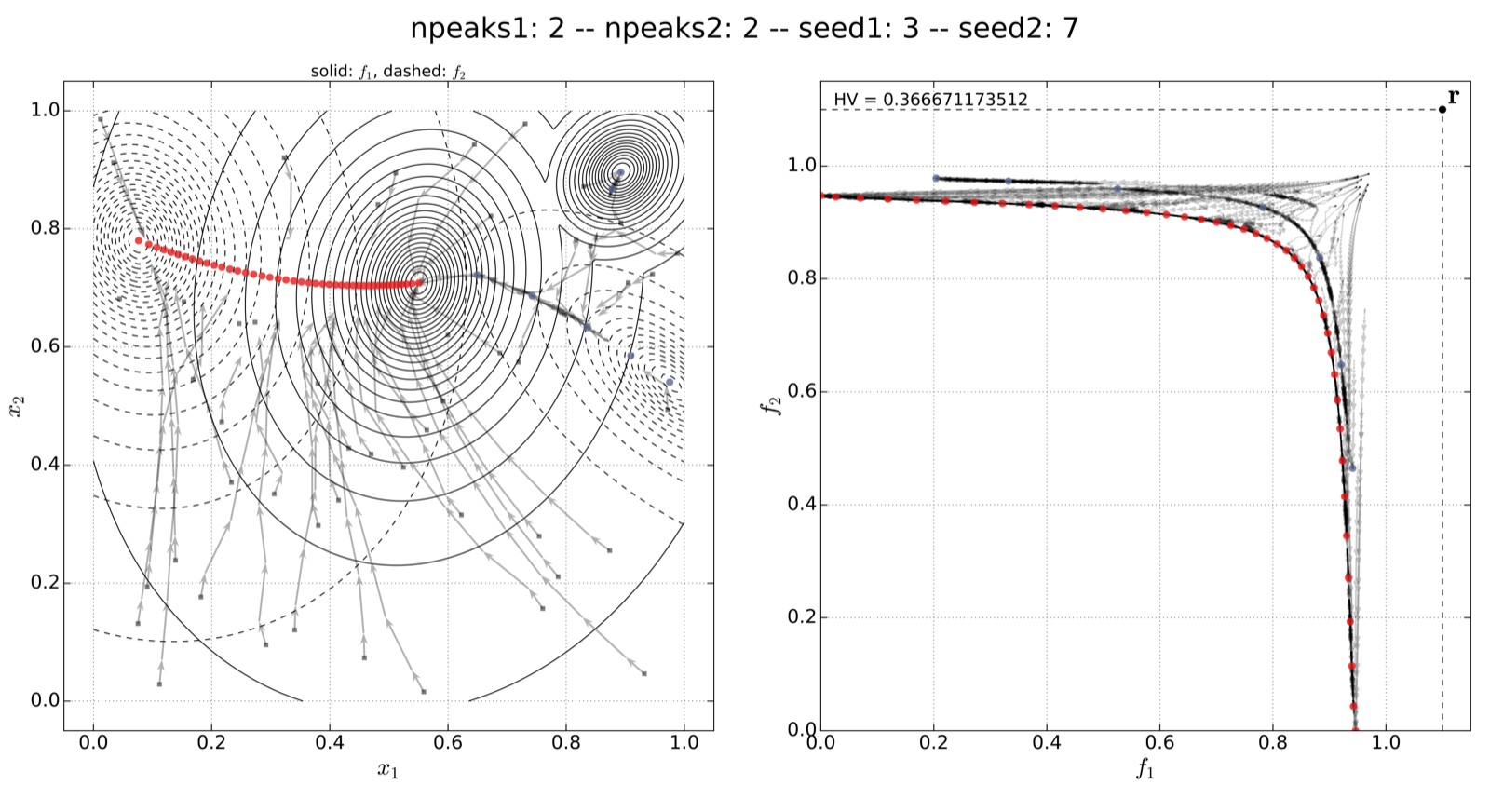
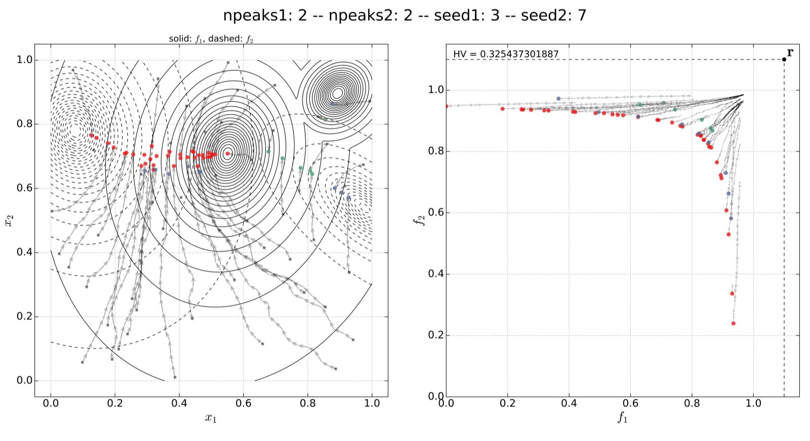
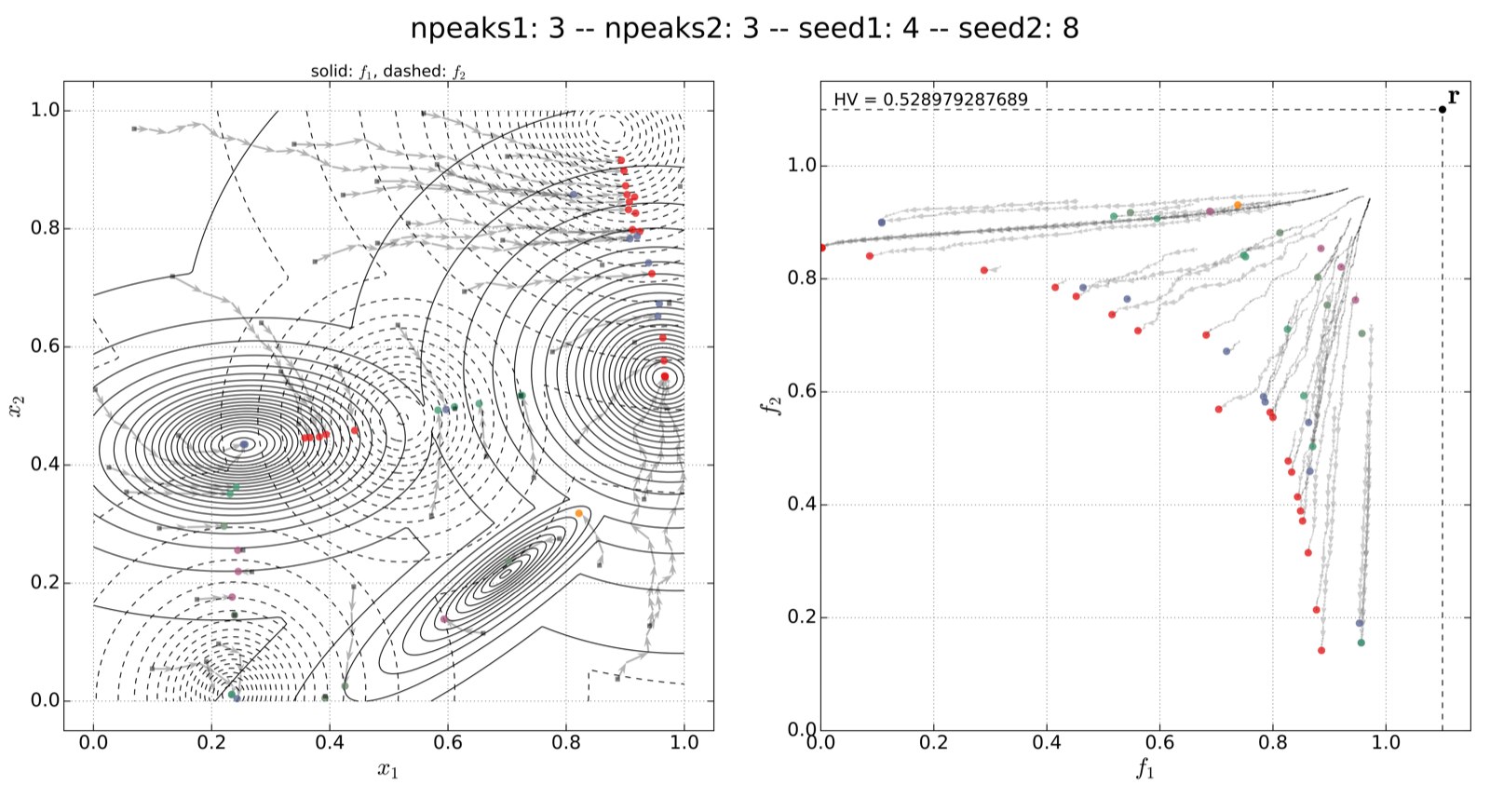
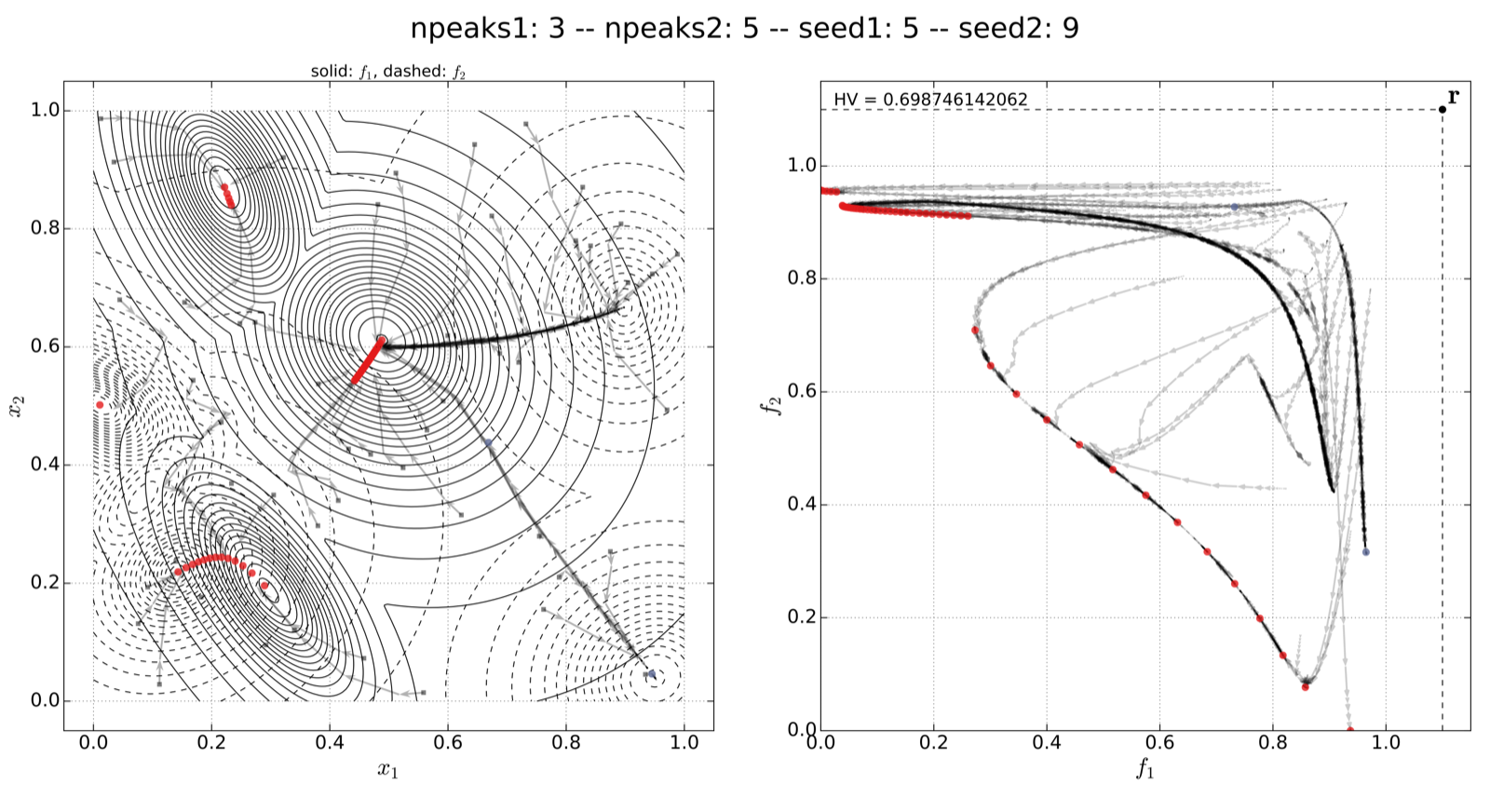
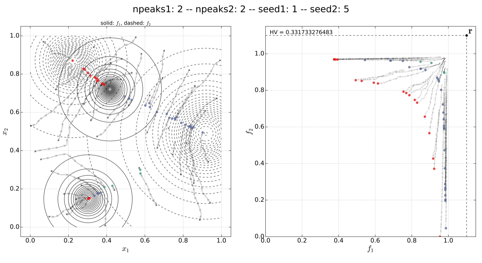
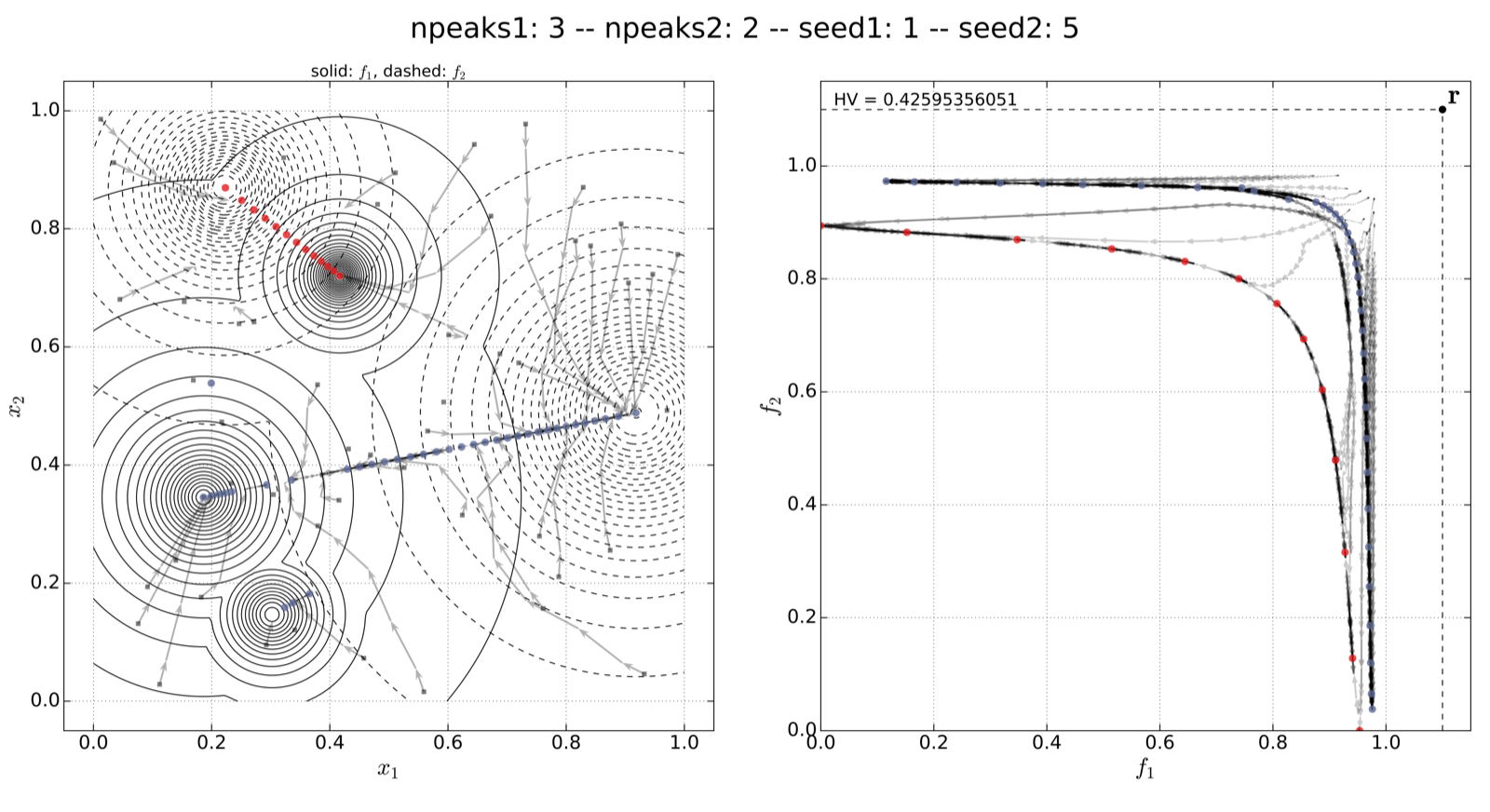
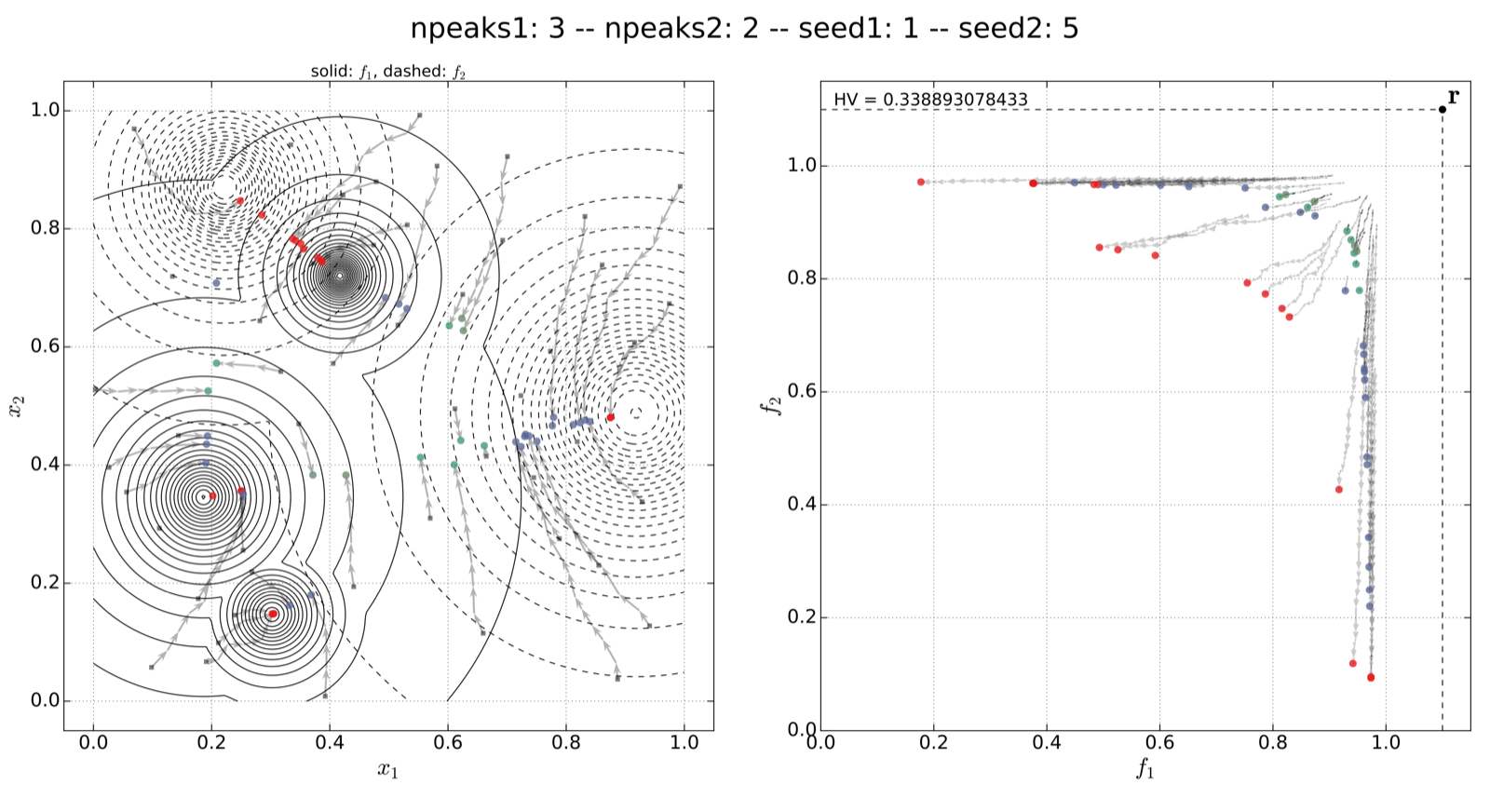
This project is based on joint work of members from our group (Information Systems and Statistics) and the "Leiden Institute of Advanced Computer Science" (LIACS). Our findings are collected in a paper called "Search Dynamics on Multimodal Multi-Objective Problems", which was accepted for publication in the Evolutionary Computation Journal (ECJ) in September 2018. The manuscript combines and extends work from our (best) paper on "Towards Analyzing Multimodality of Multiobjective Landscapes" (published at the 14th International Conference on Parallel Problem Solving from Nature (PPSN XIV)), as well as our papers on "An Expedition to Multimodal Multi-Objective Optimization Landscapes" and "Hypervolume Indicator Gradient Ascent Multi-objective Optimization", both published at the 9th International Conference on Evolutionary Multi-Criterion Optimization (EMO 2017).
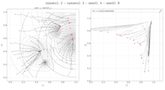
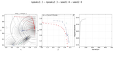
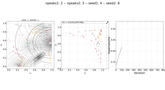
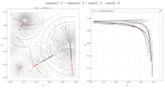
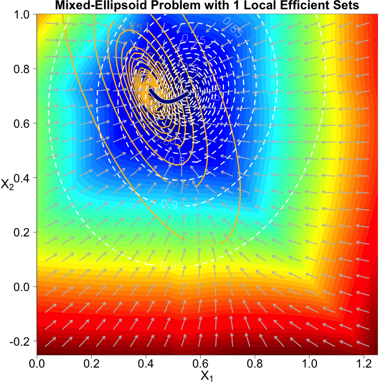
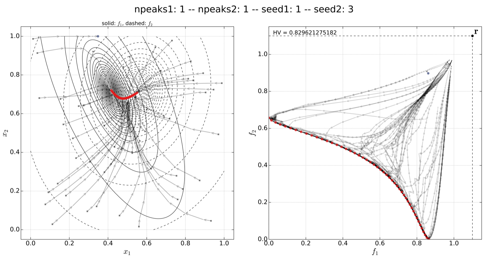
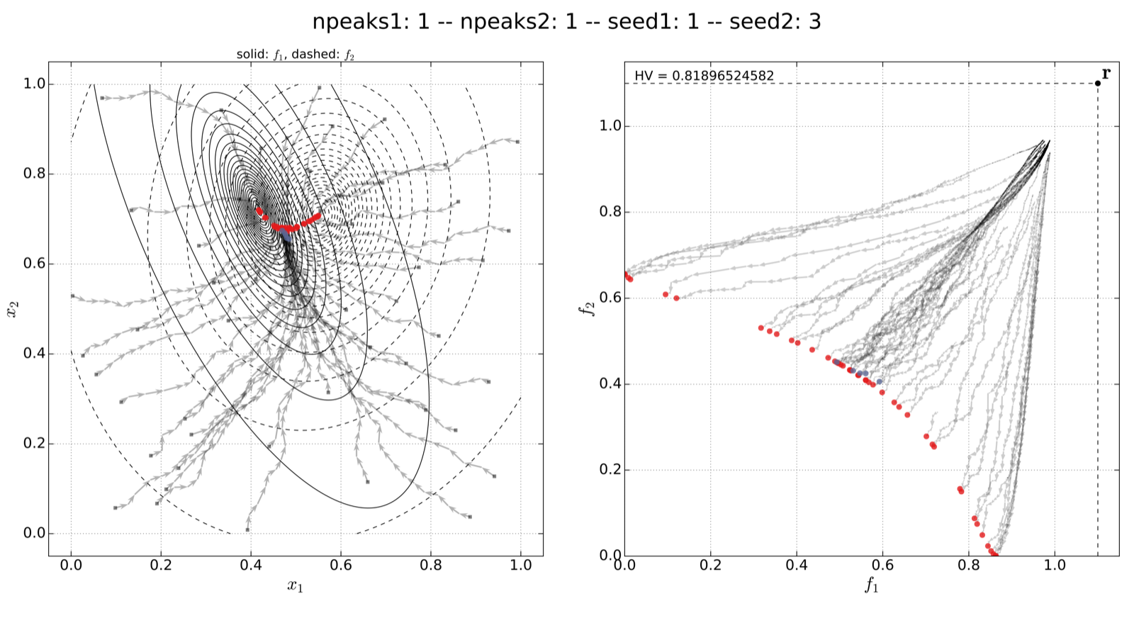
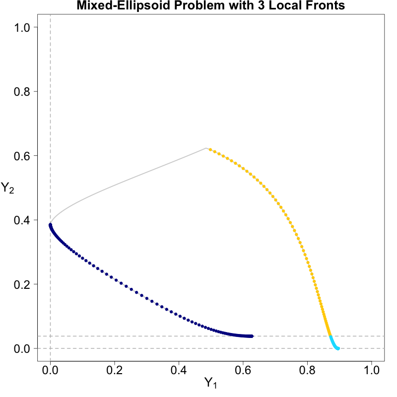
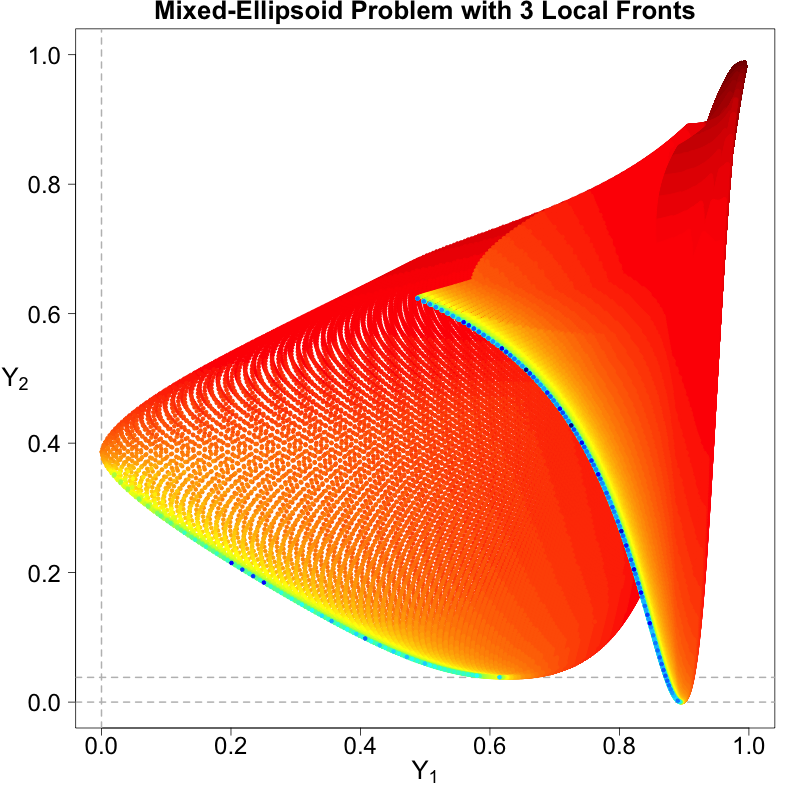
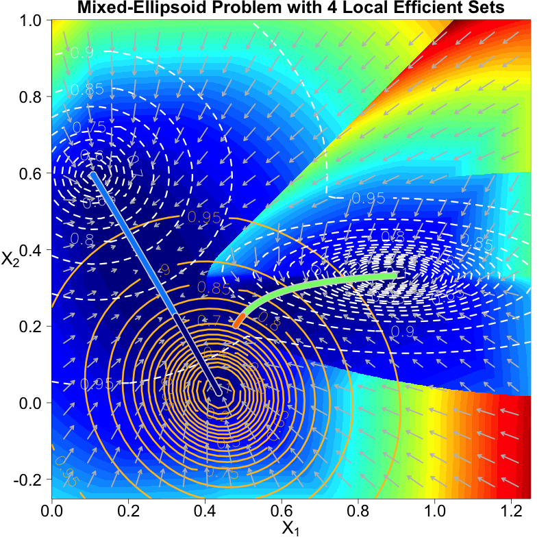
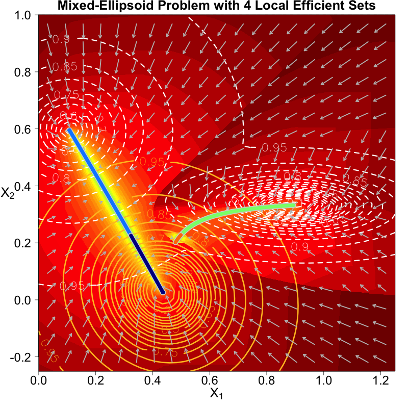
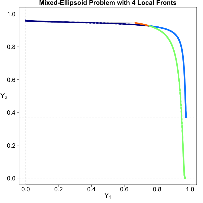
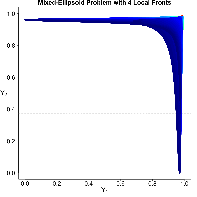
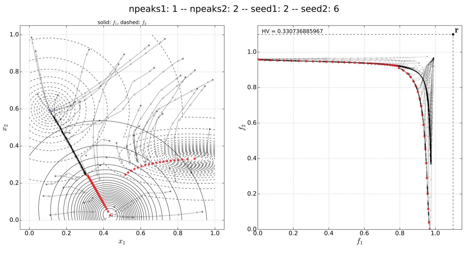
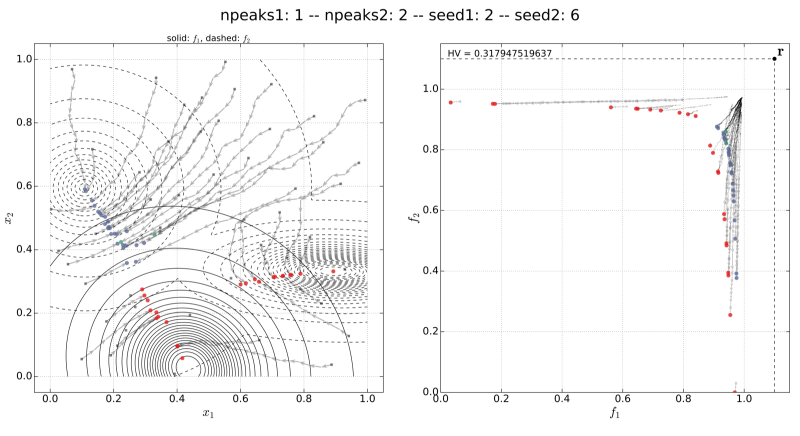
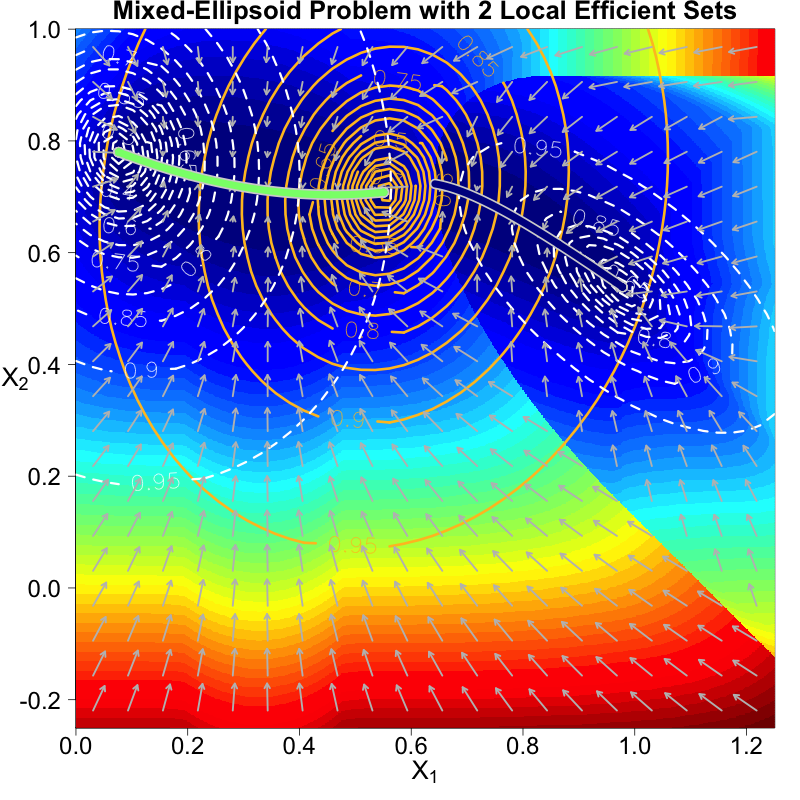
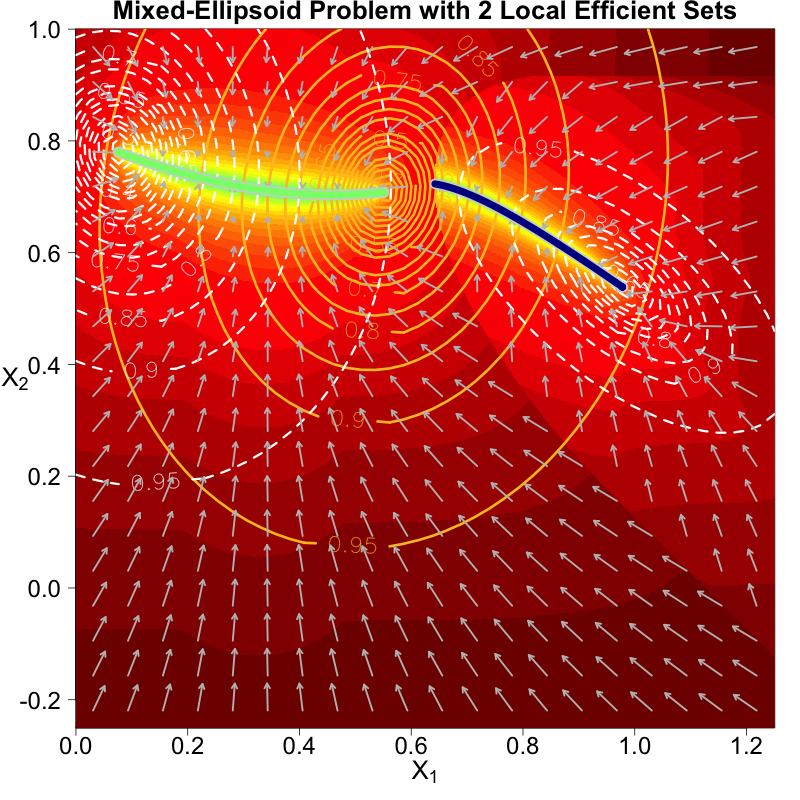
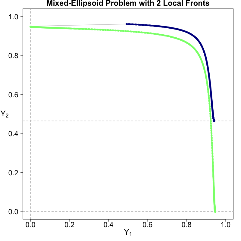
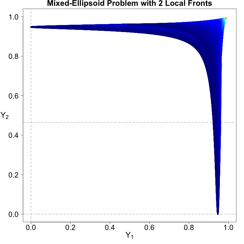
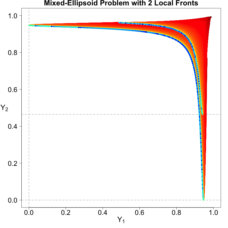
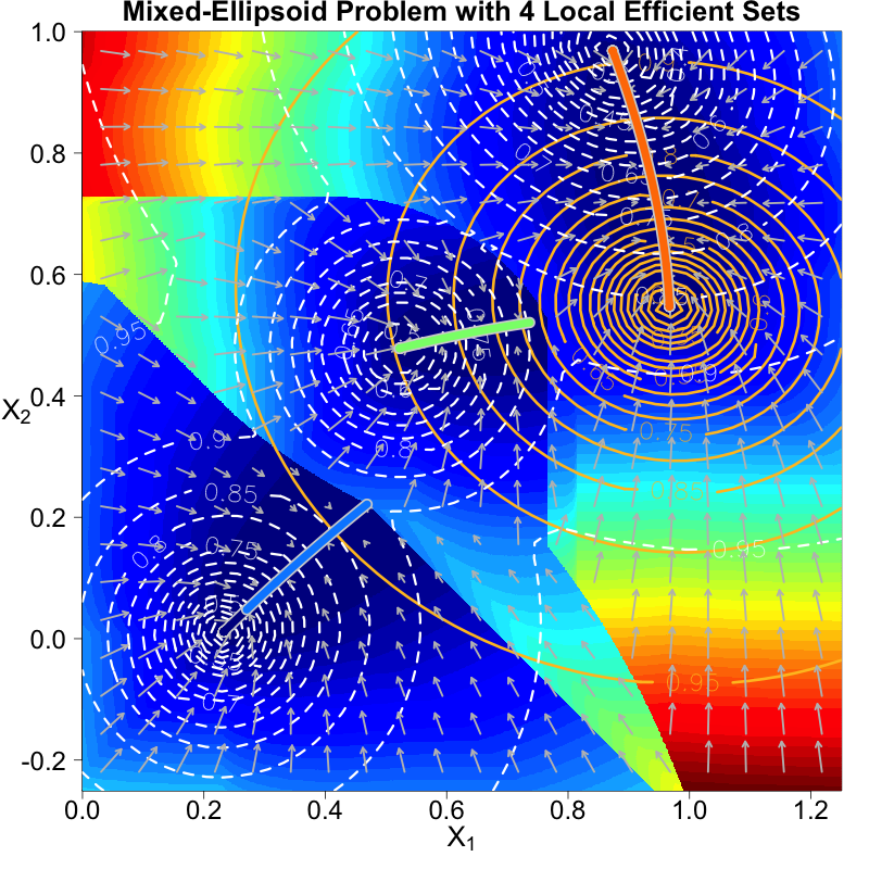
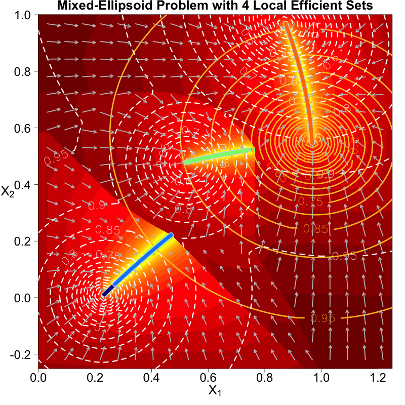
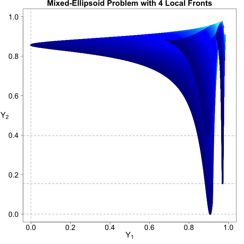
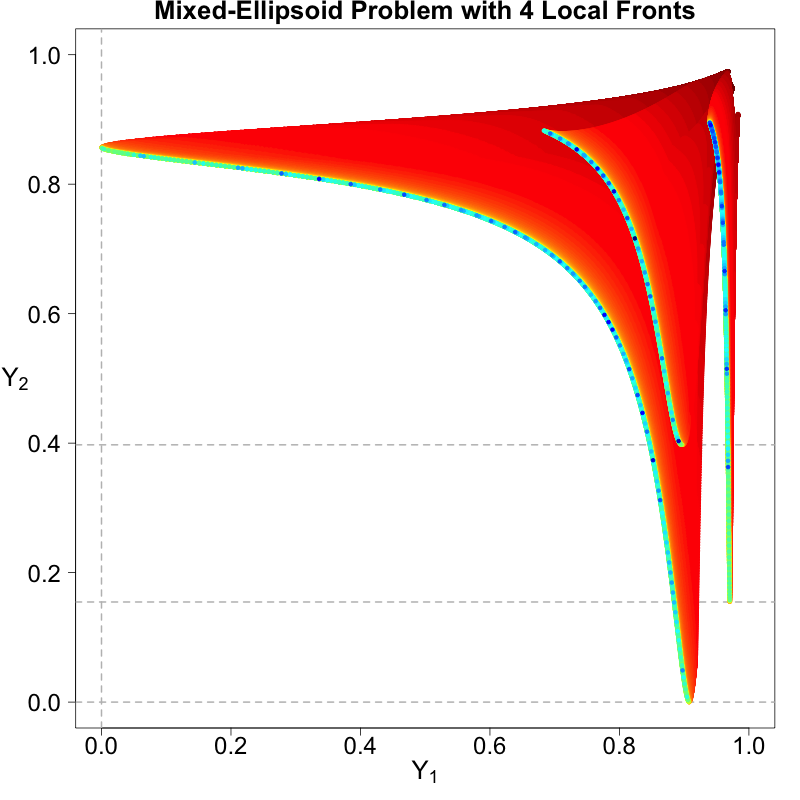
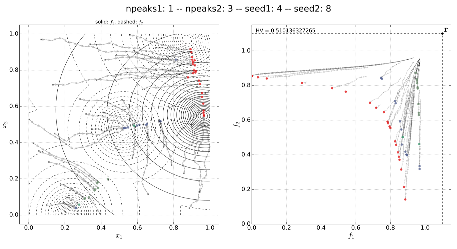
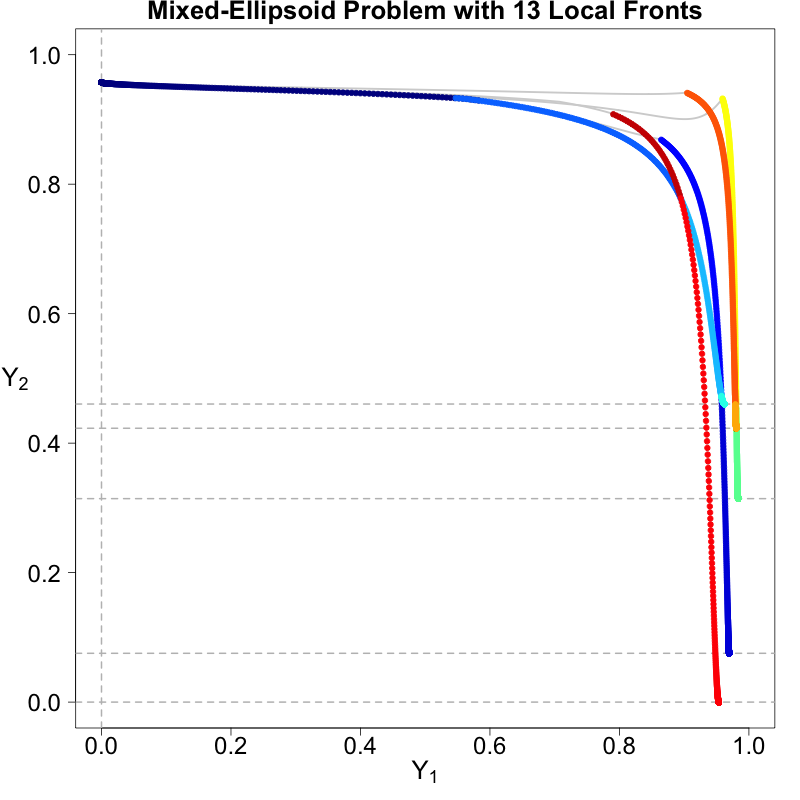
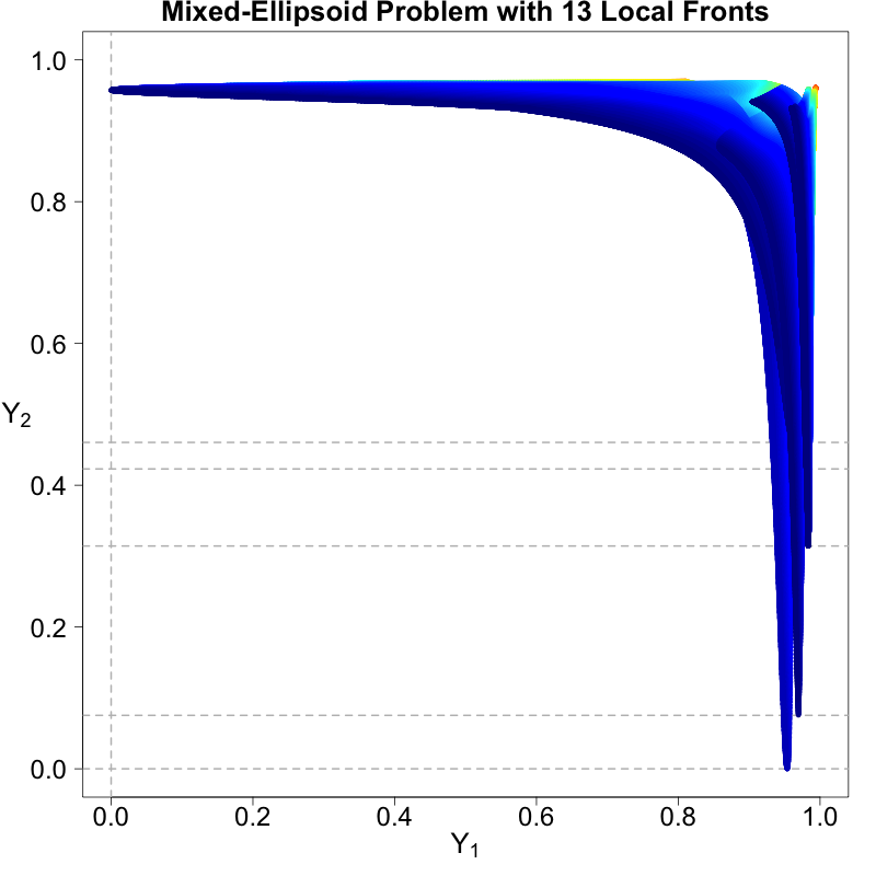
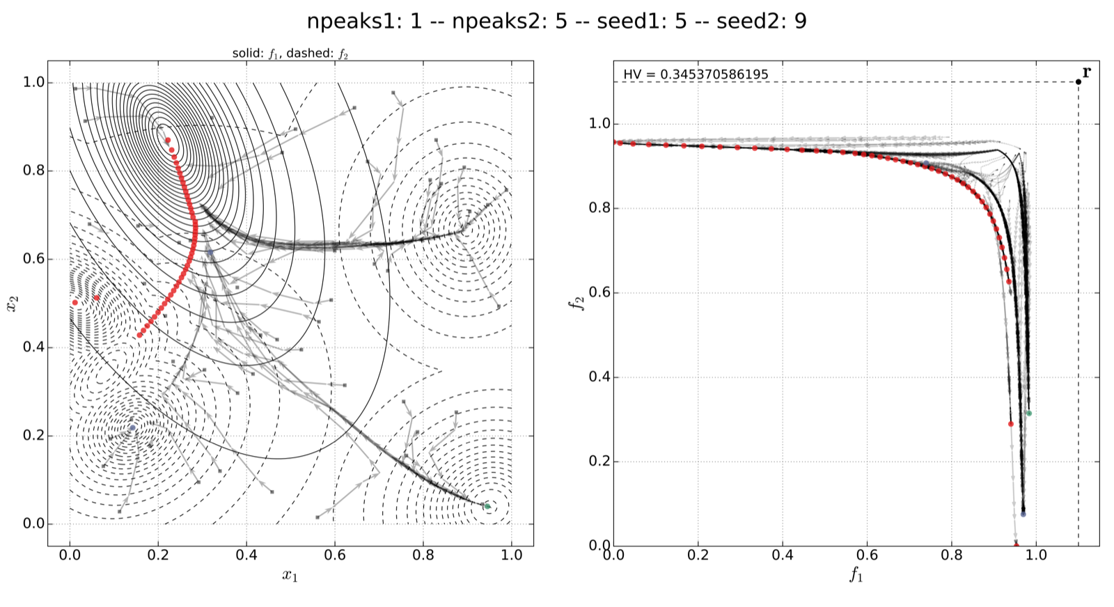
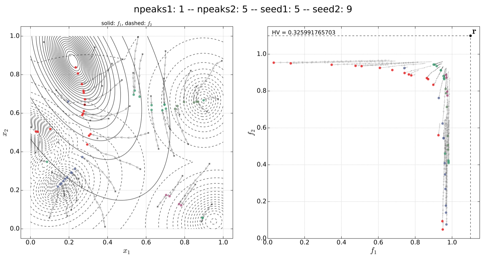
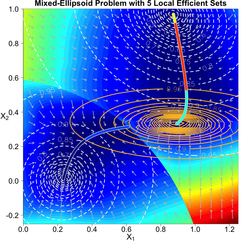
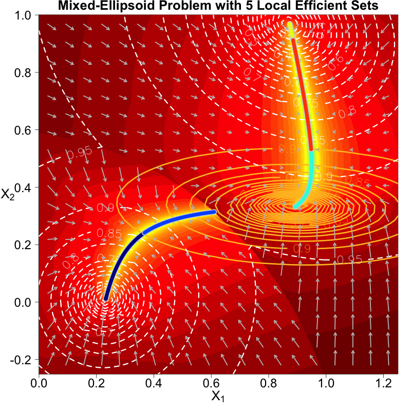
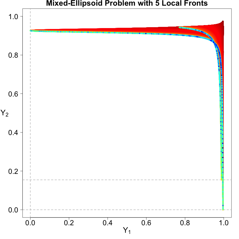
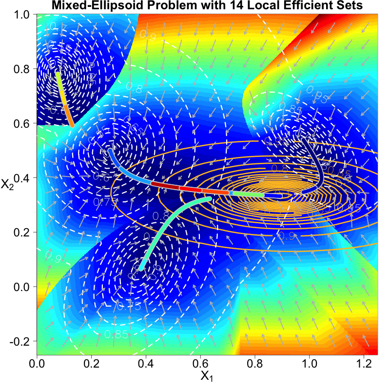
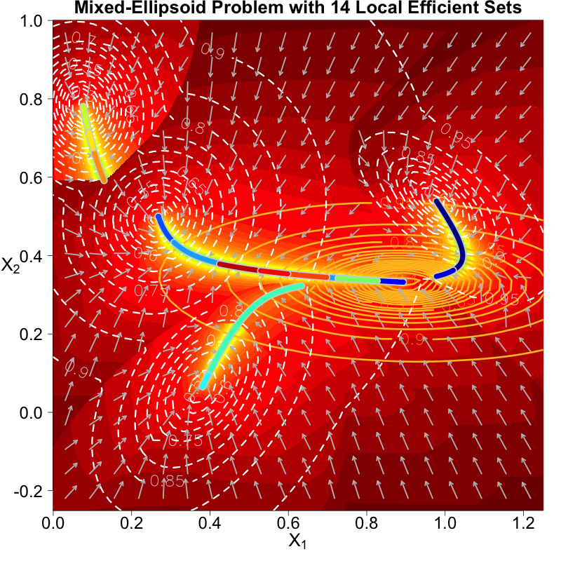
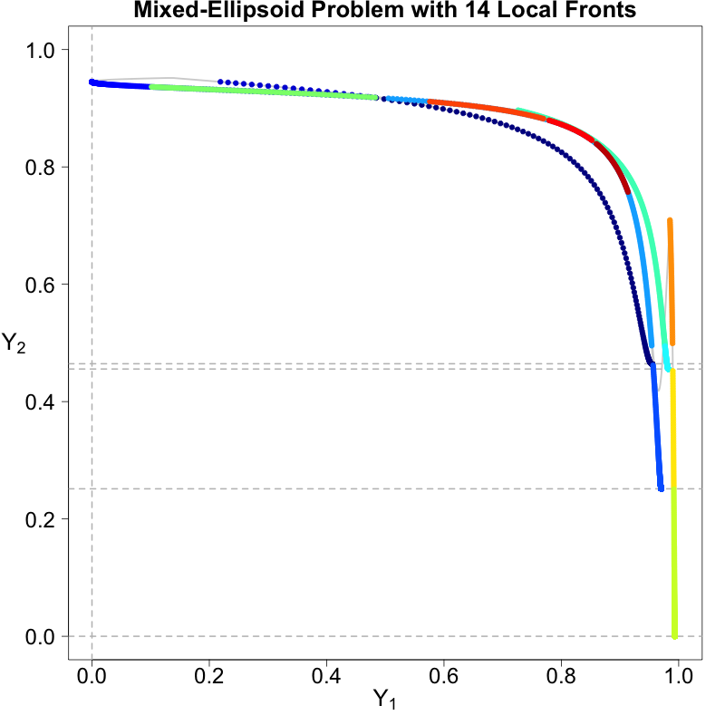
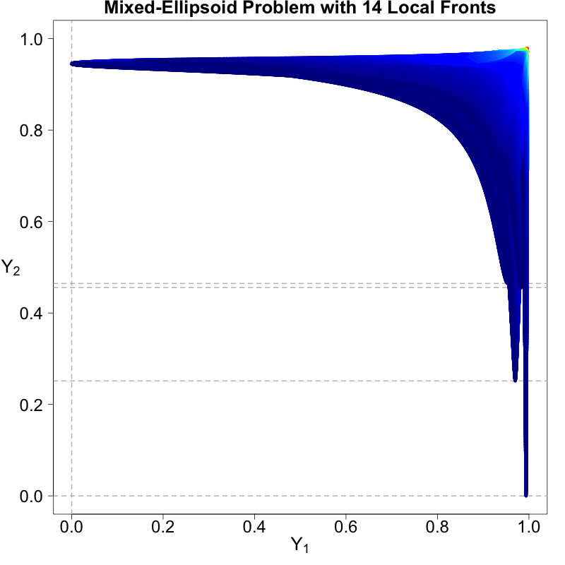
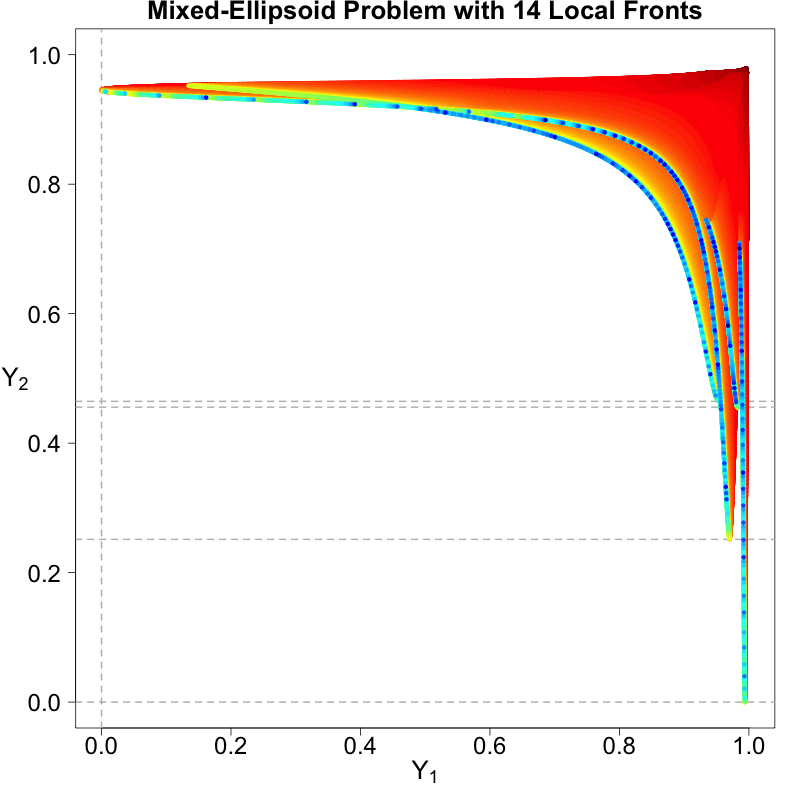
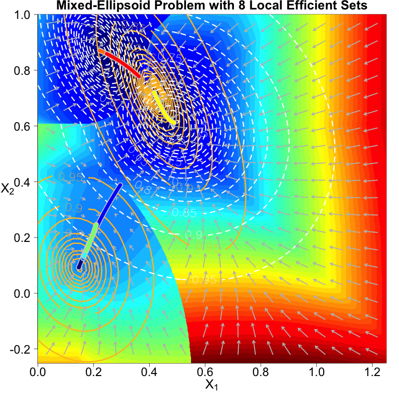
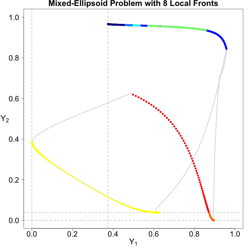
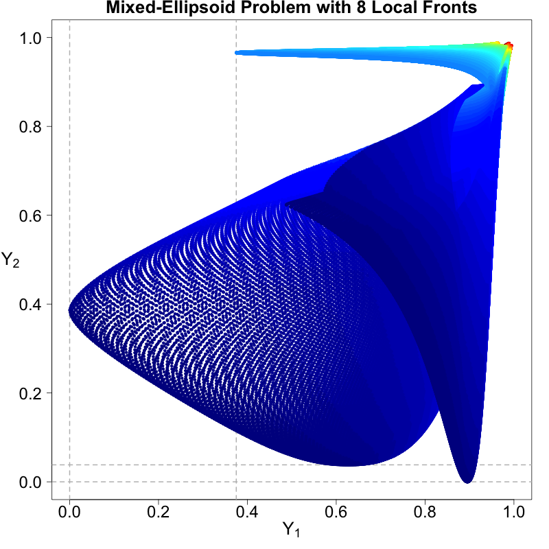
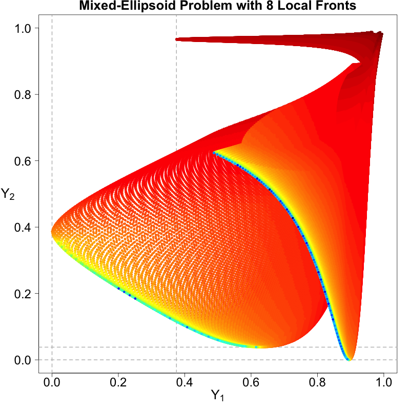
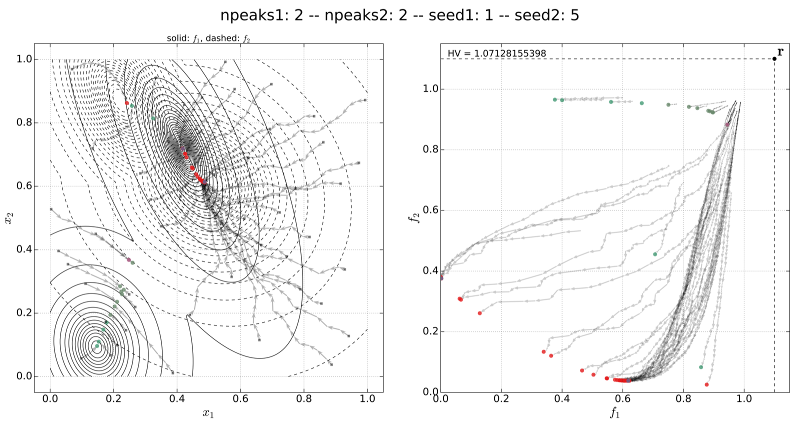
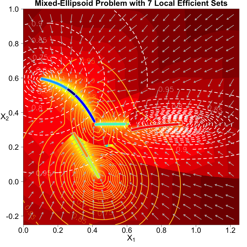
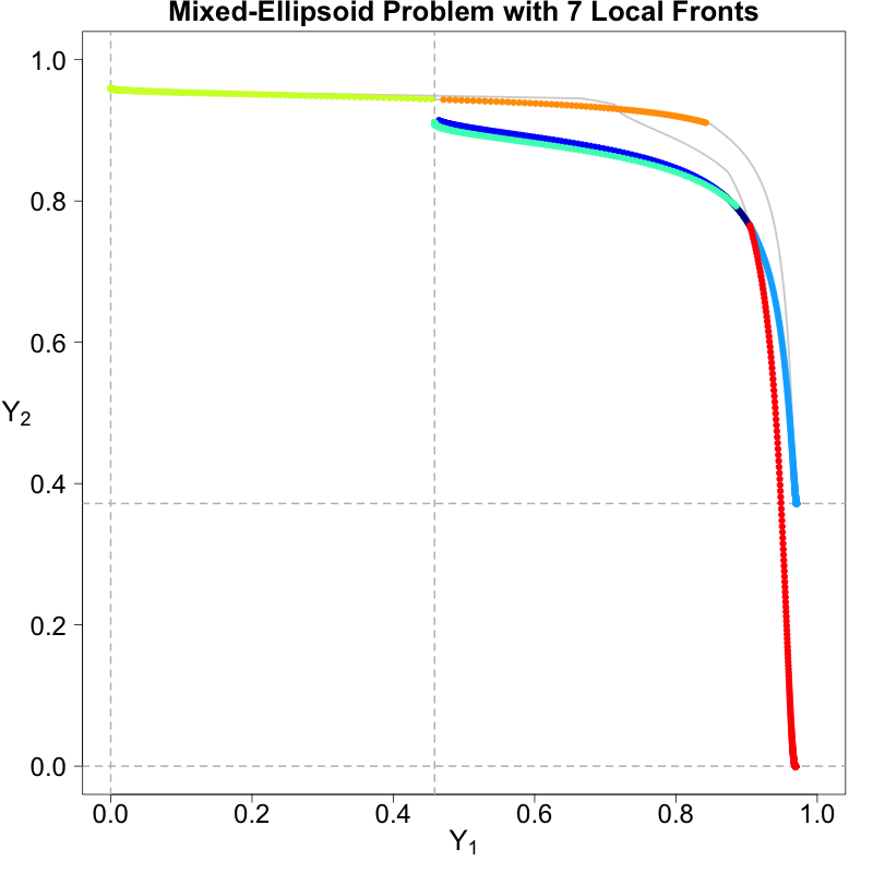
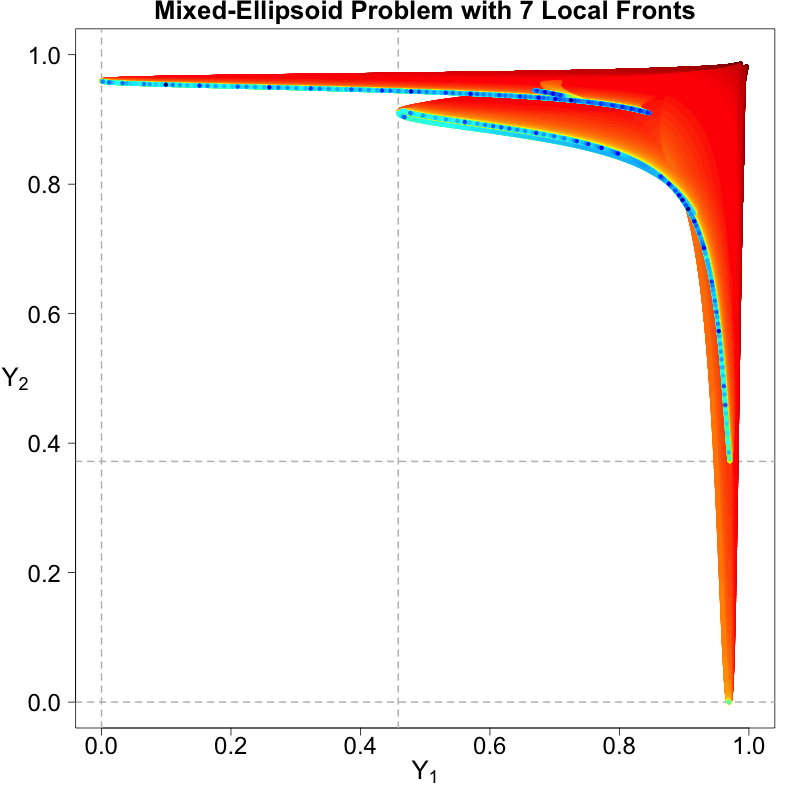
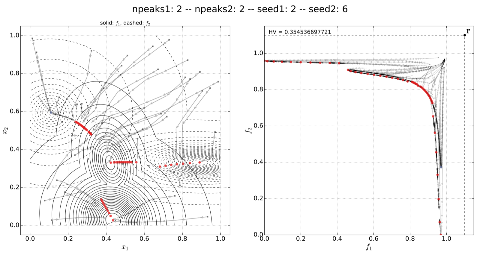
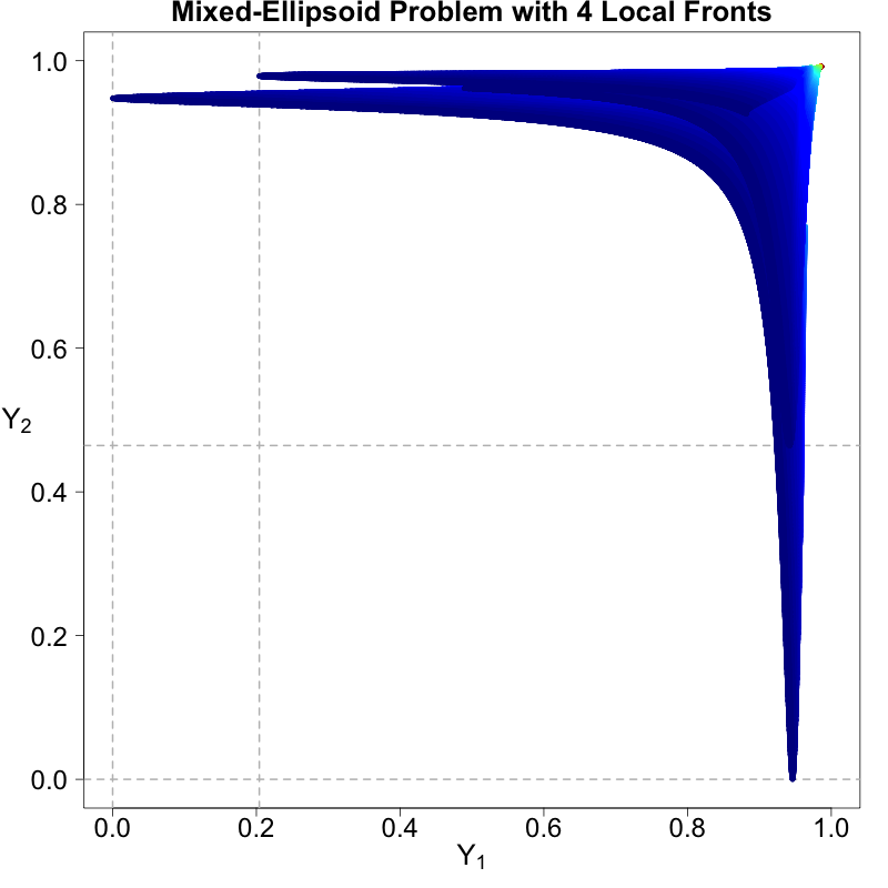
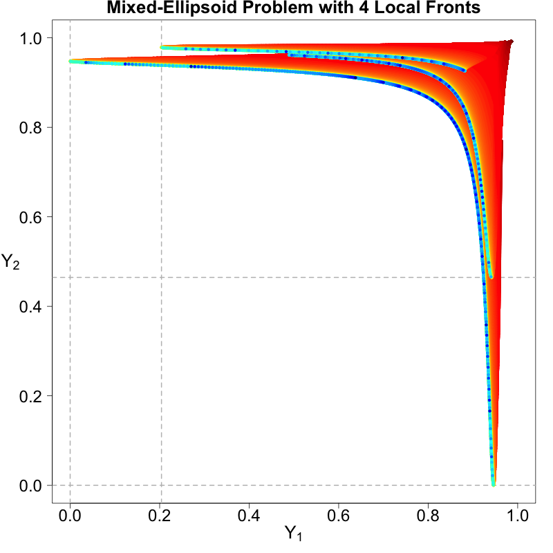
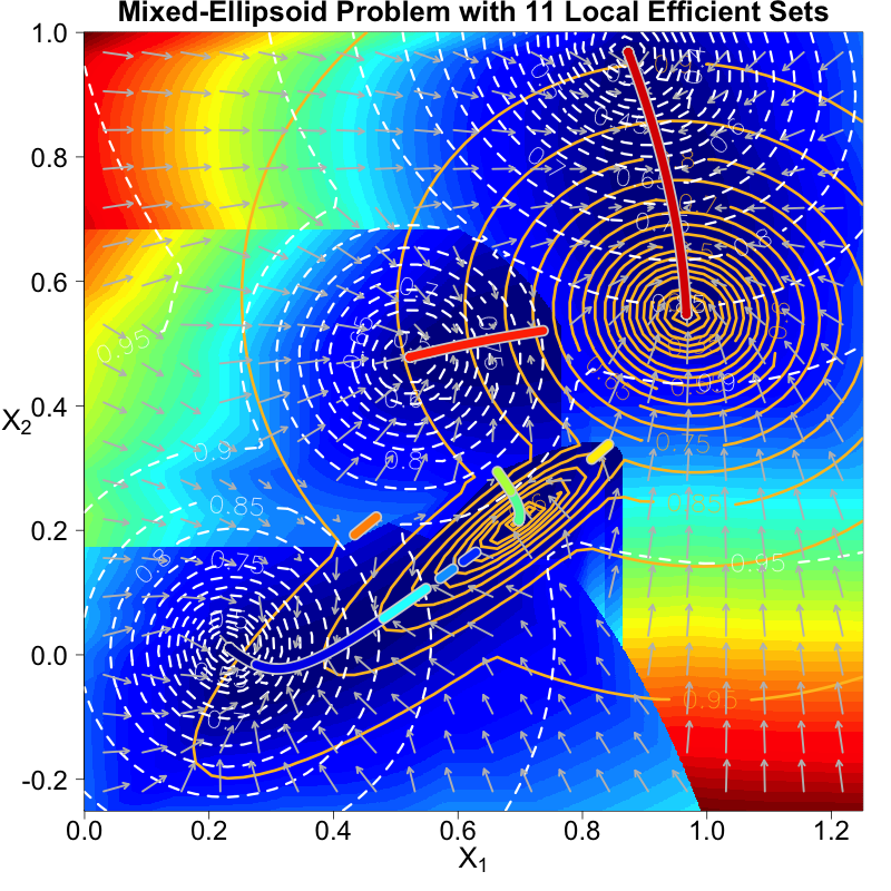
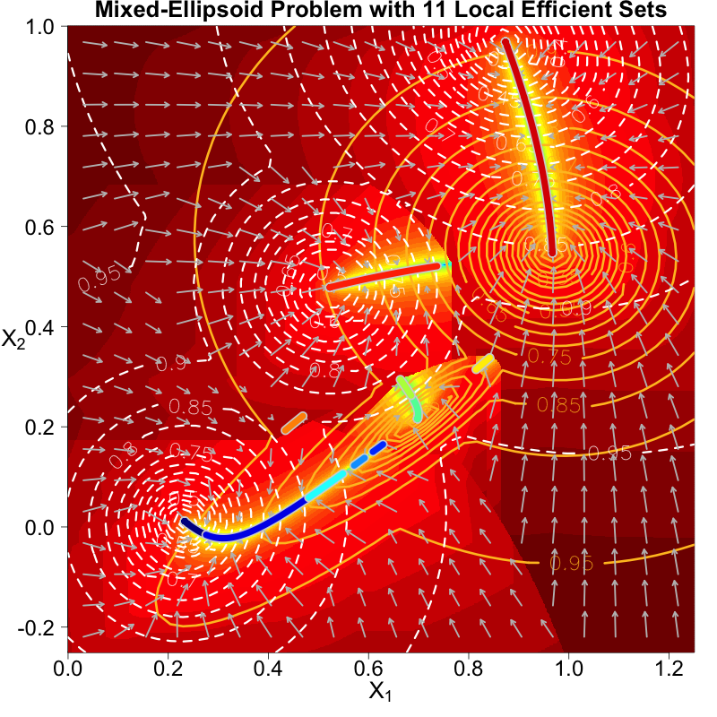
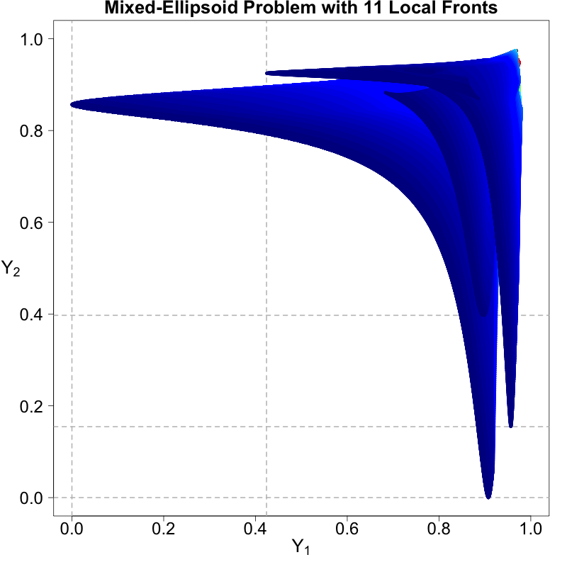
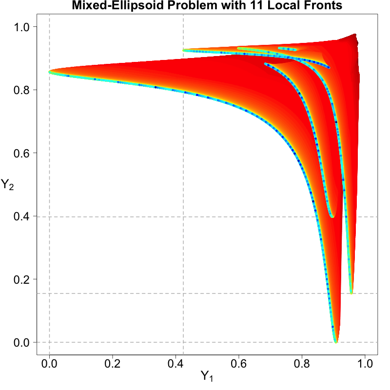
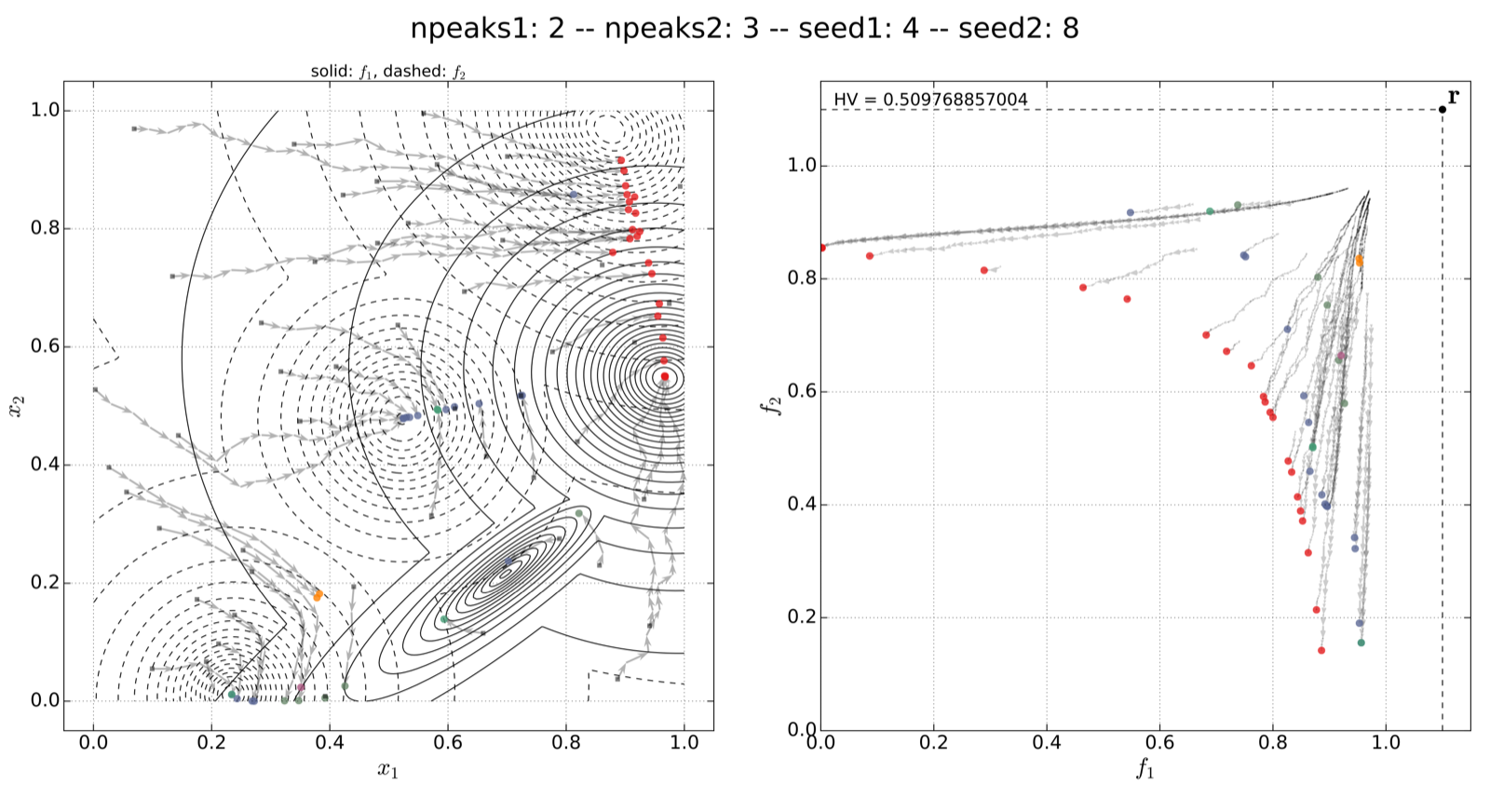
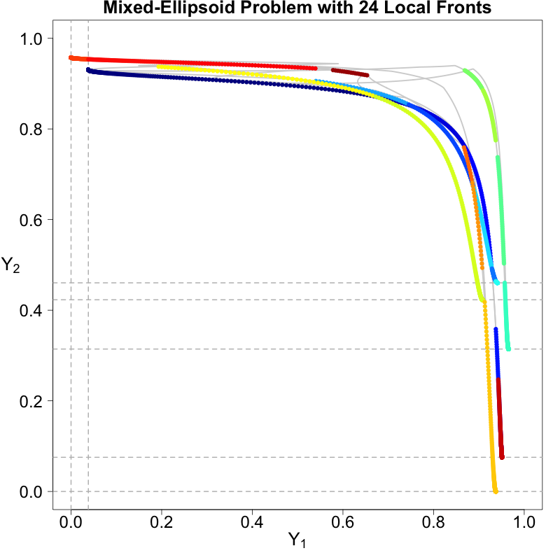
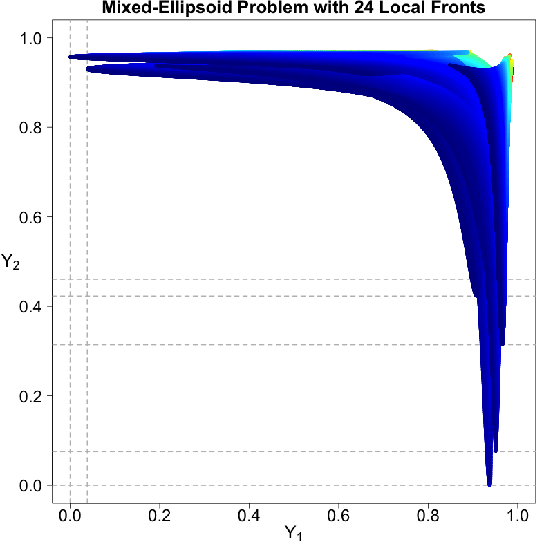
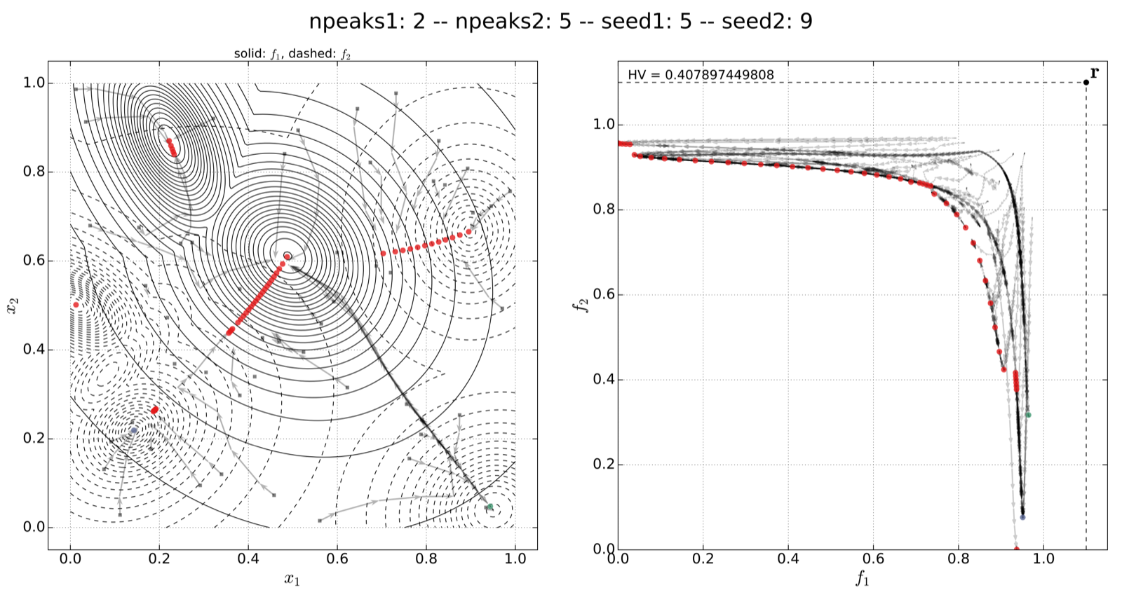
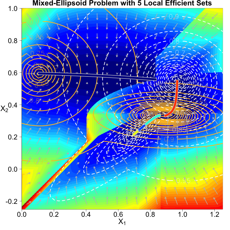
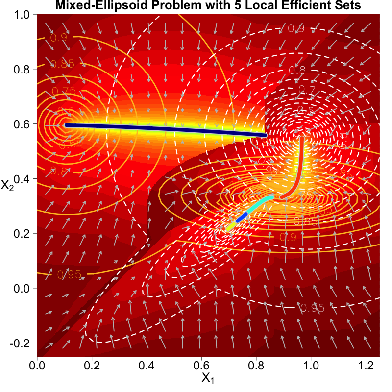
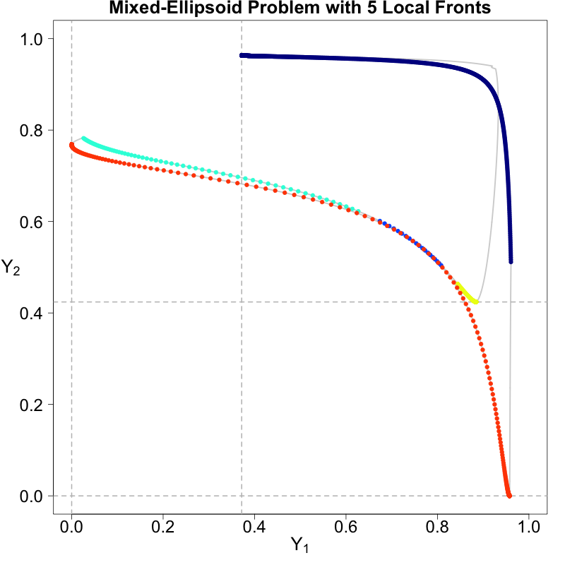
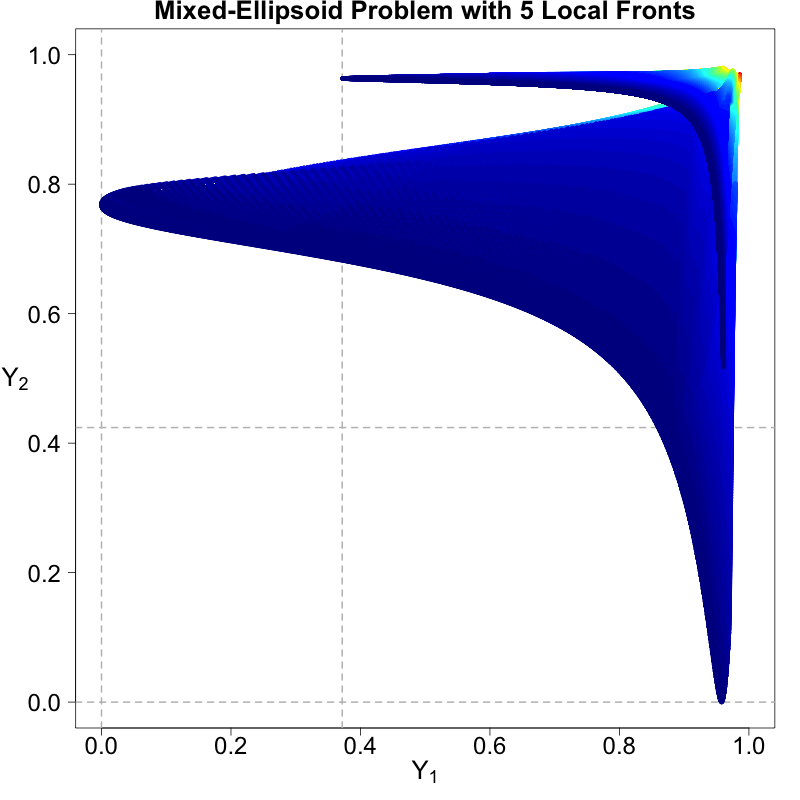
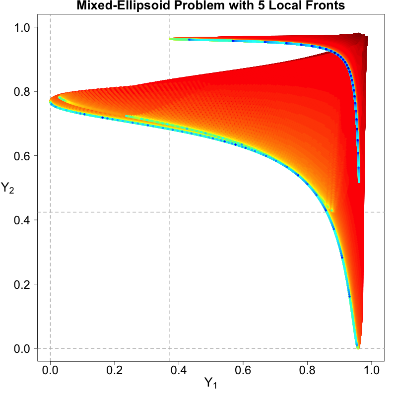
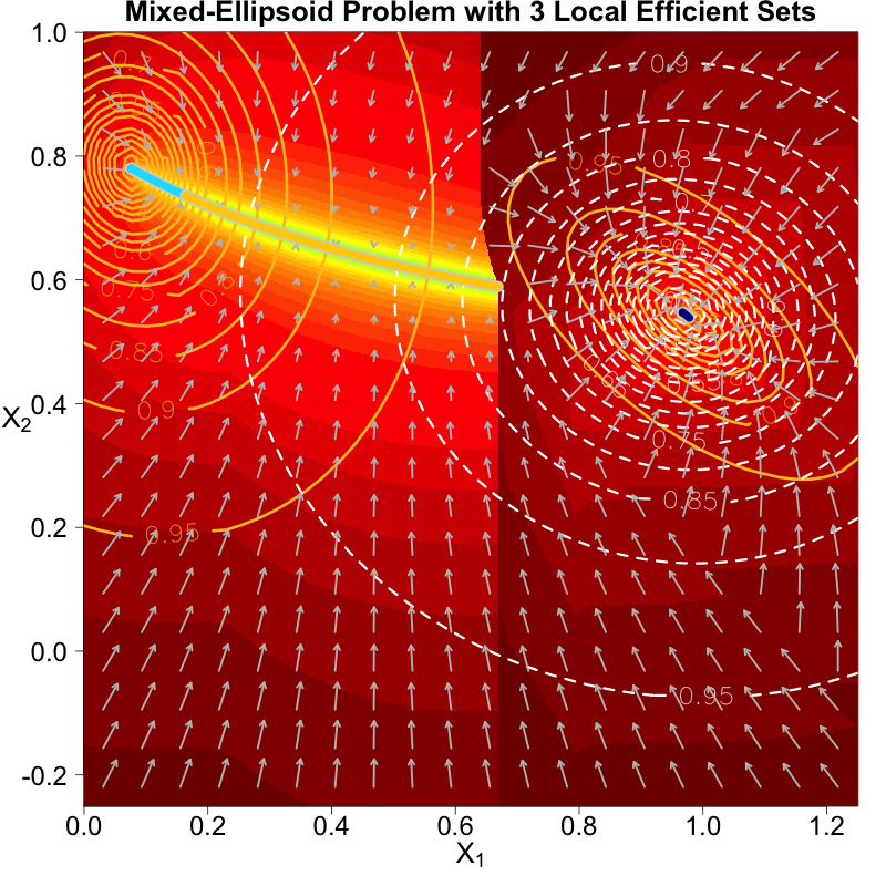
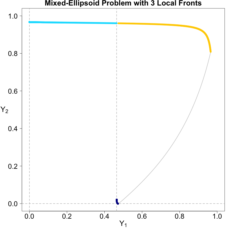
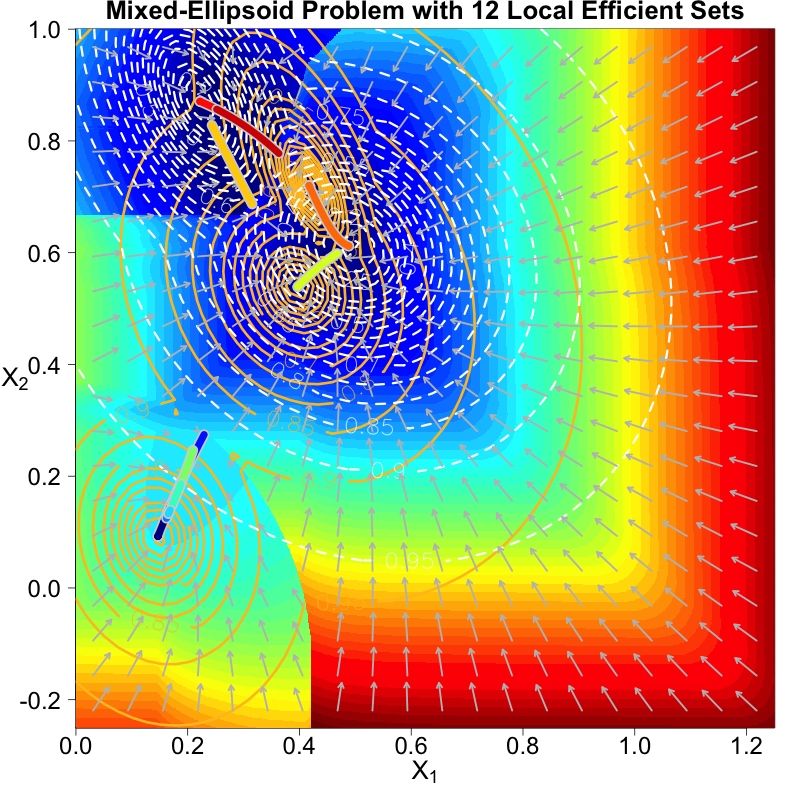
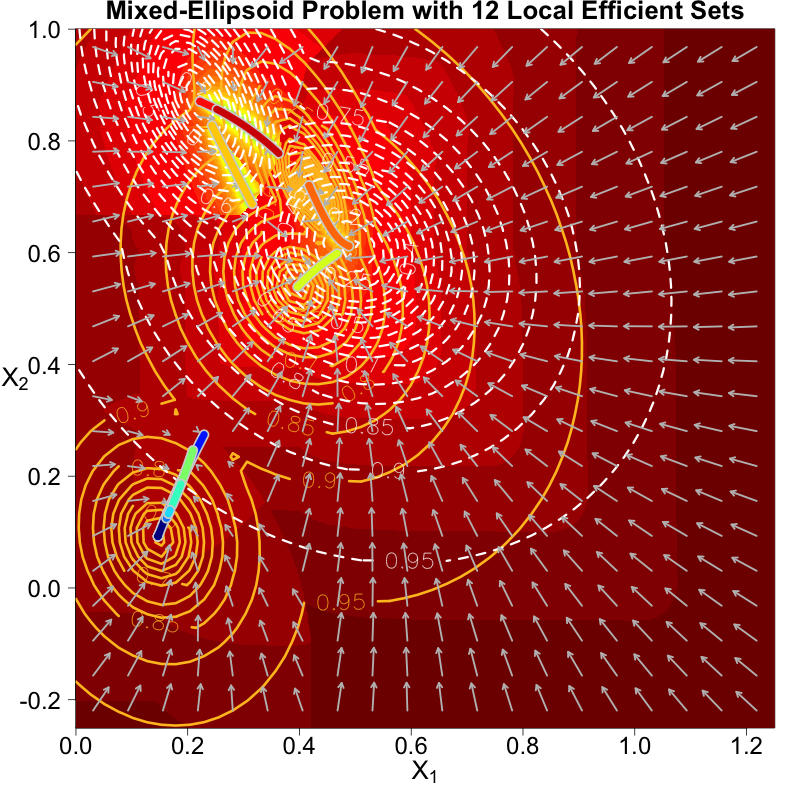
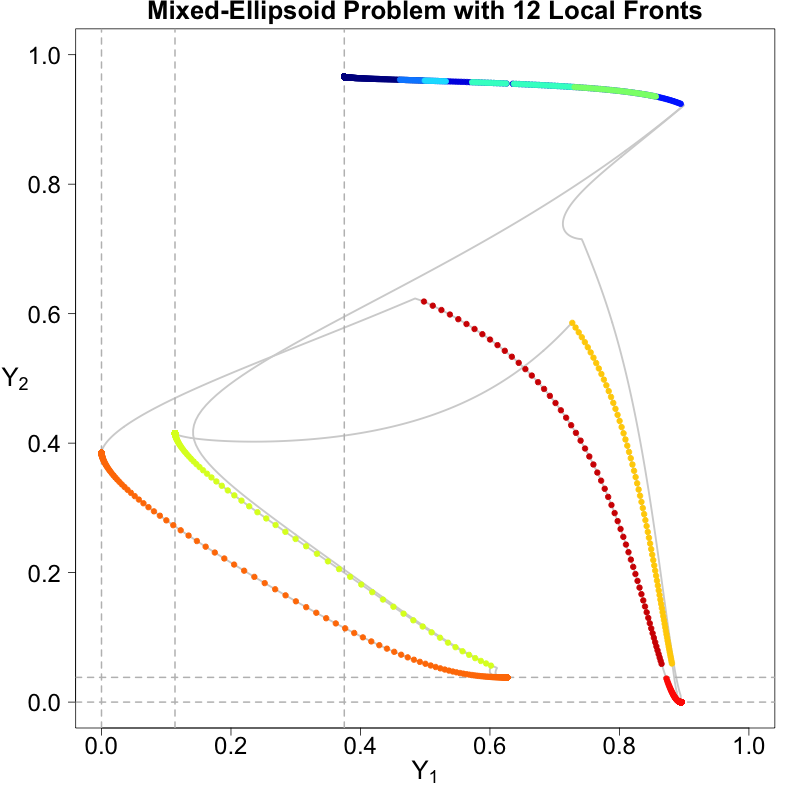
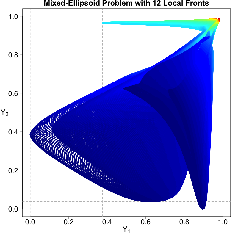
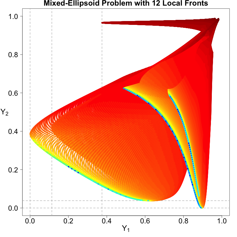
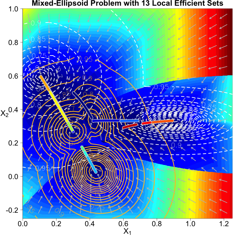
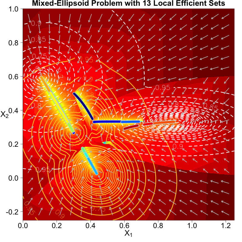
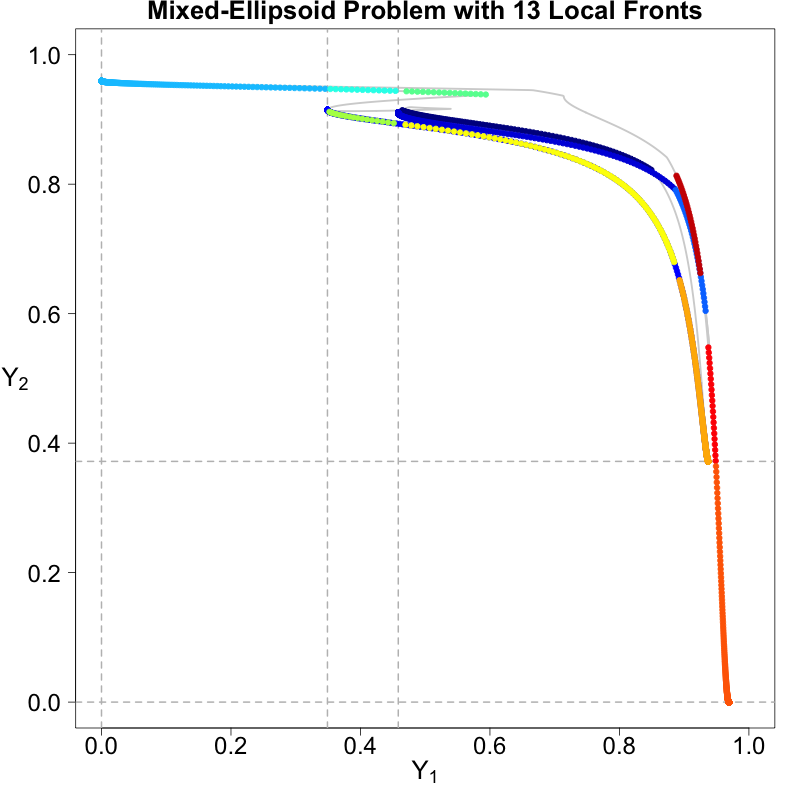
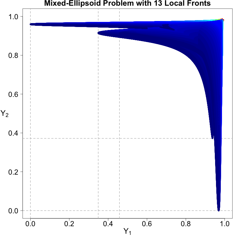
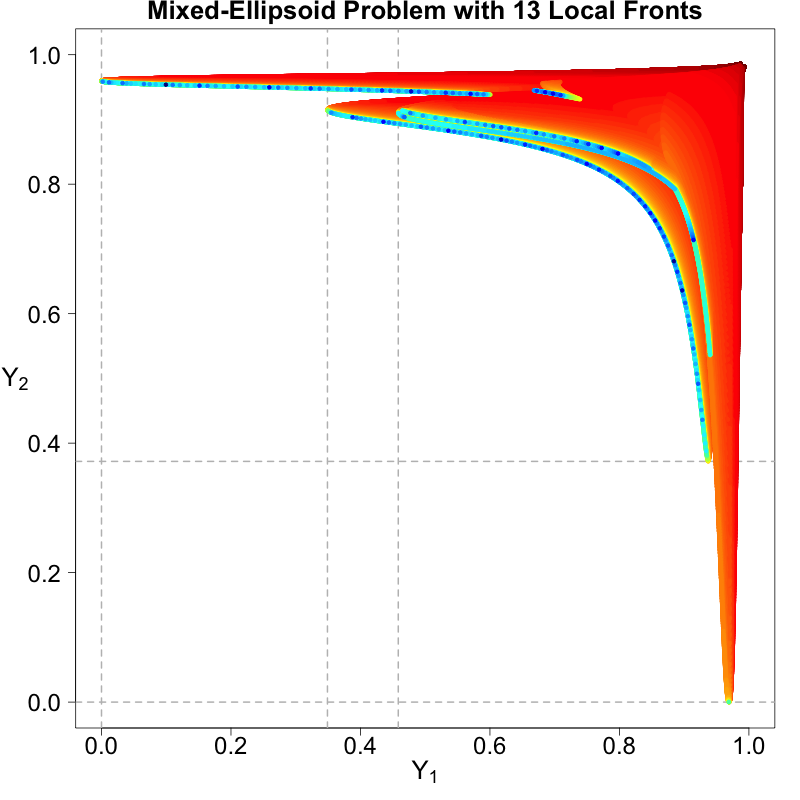
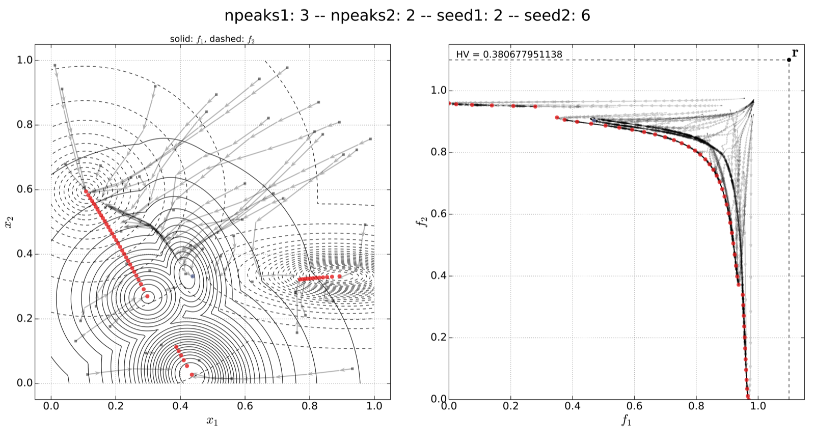
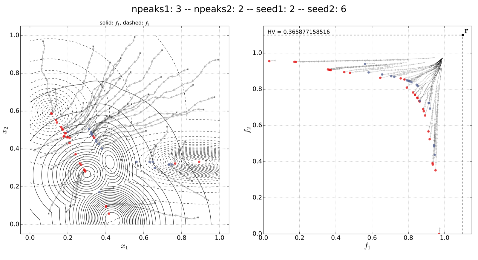
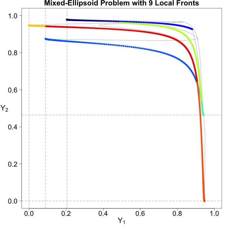
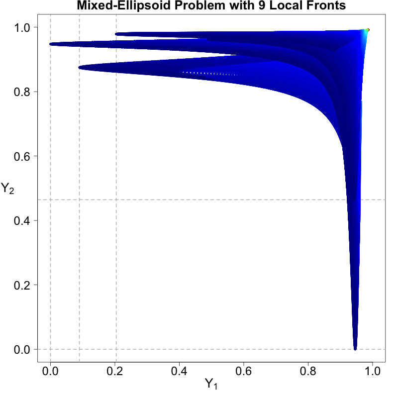
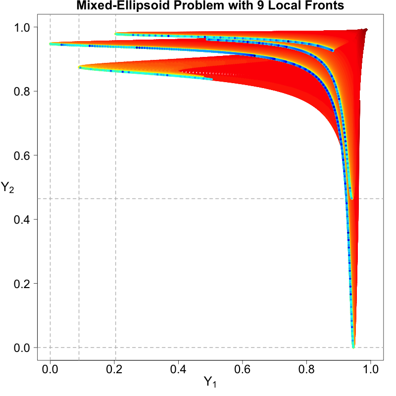
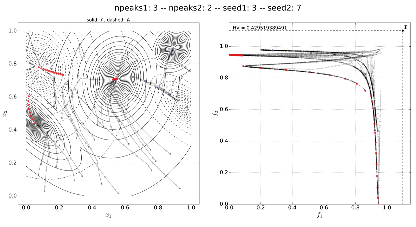
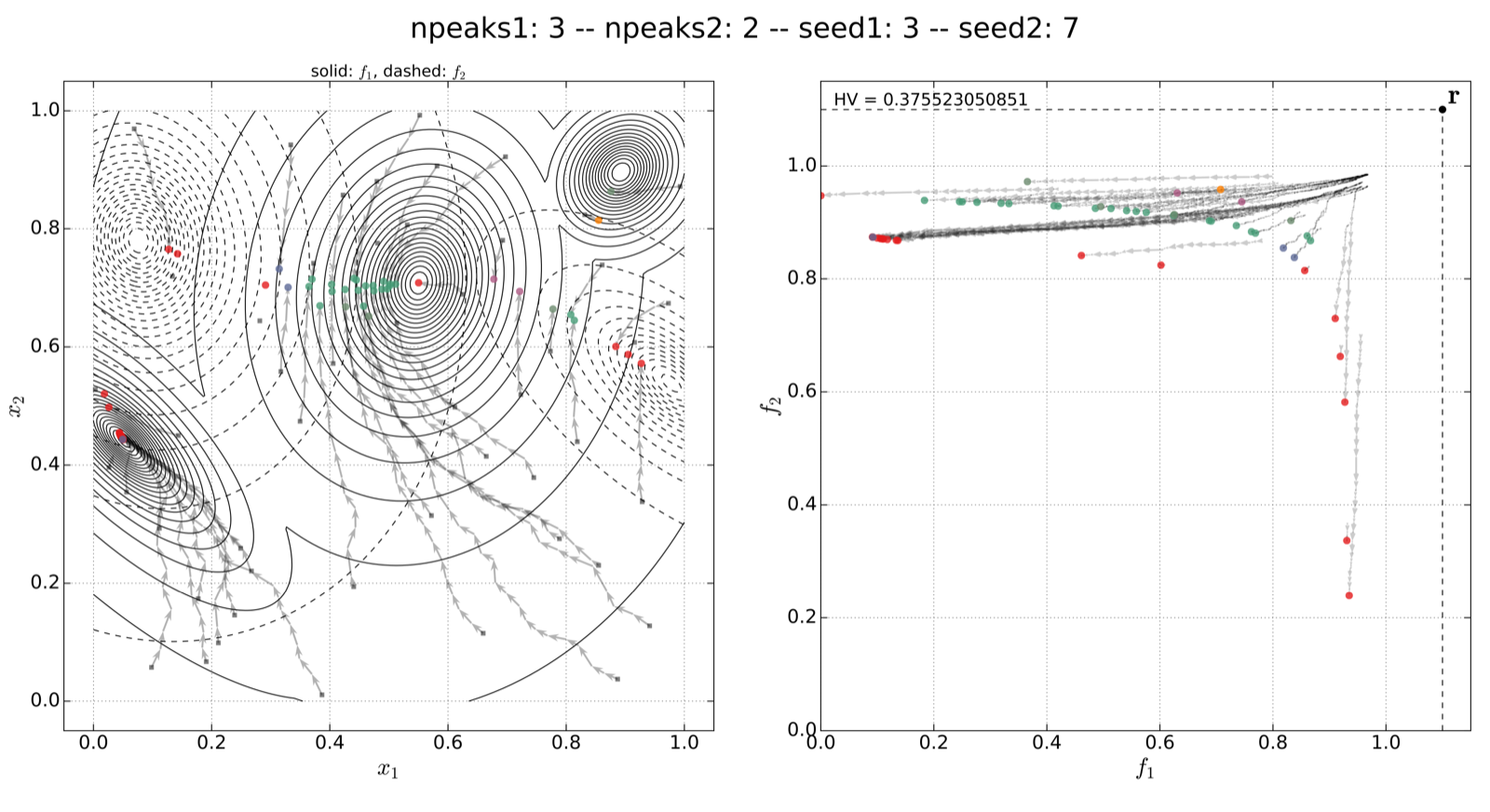
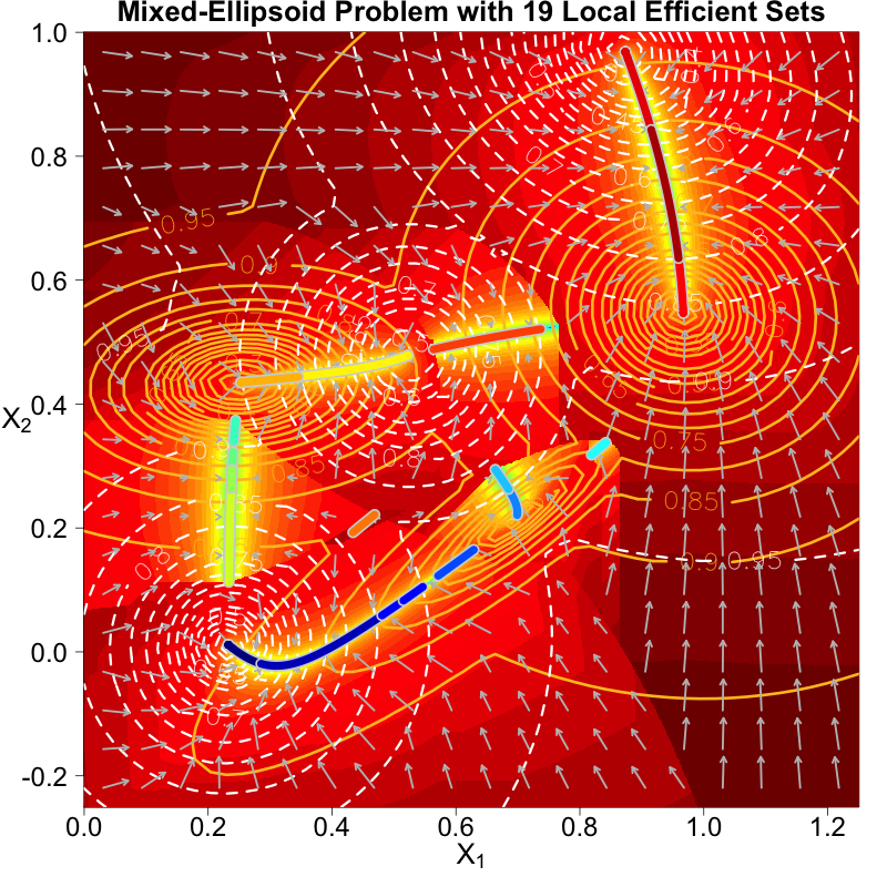
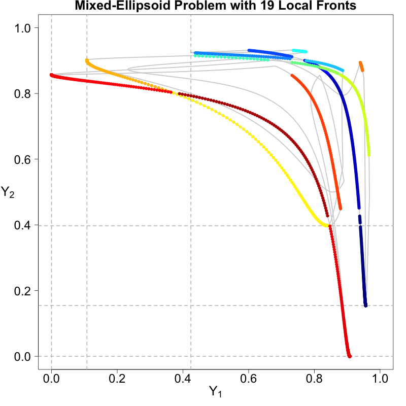
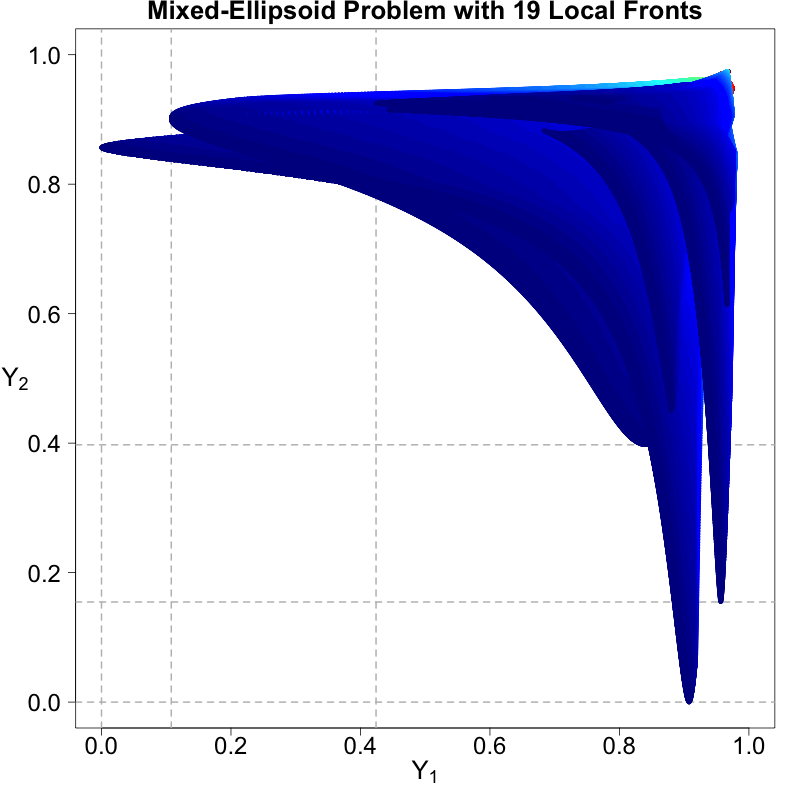
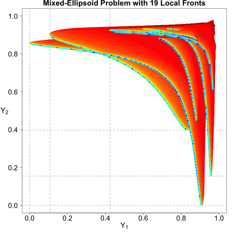
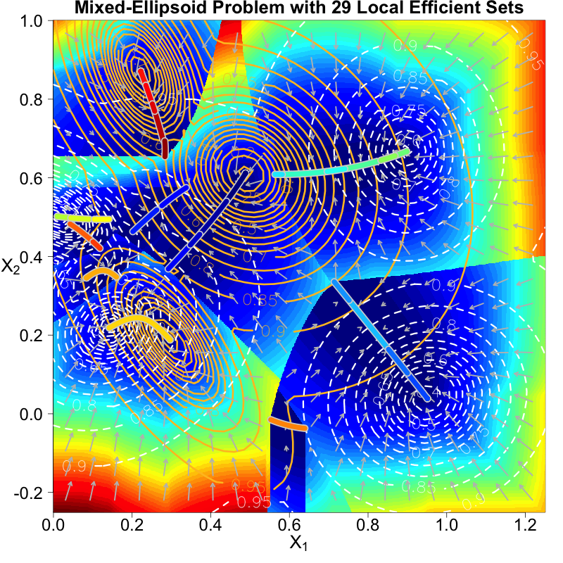
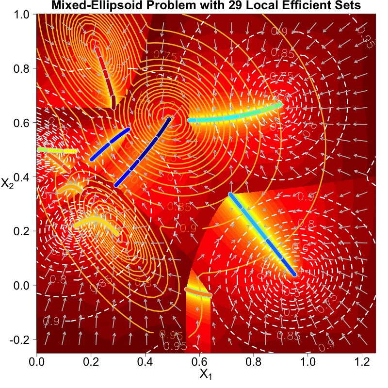
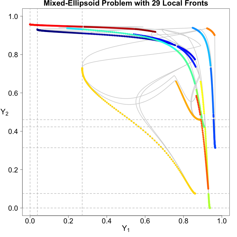
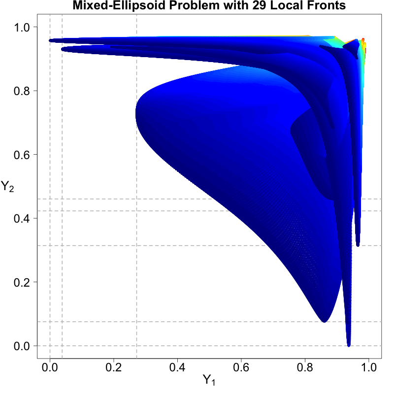
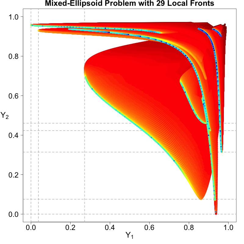
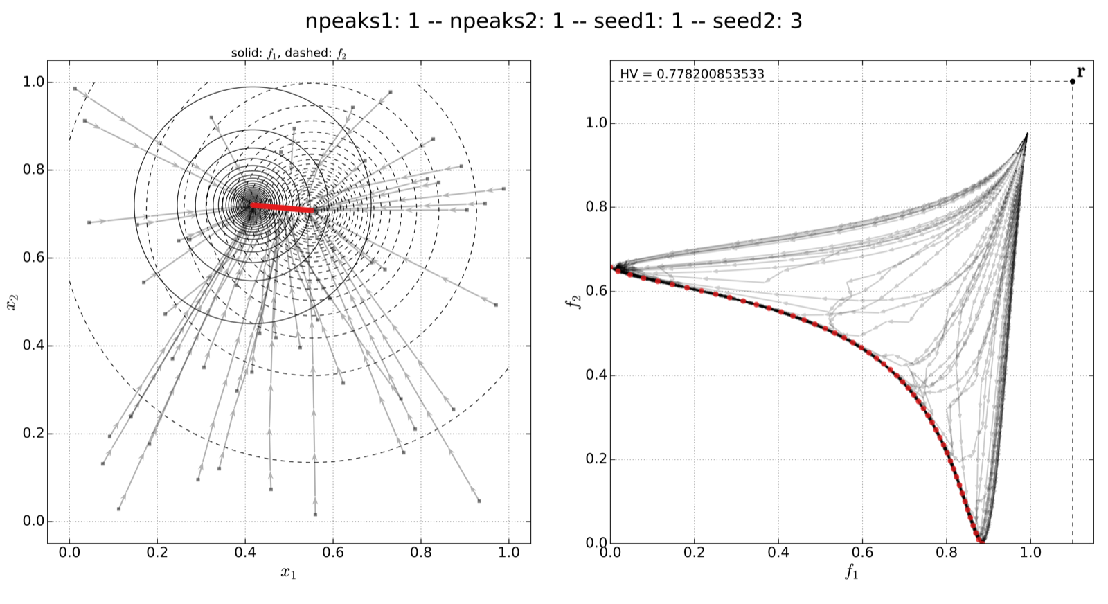
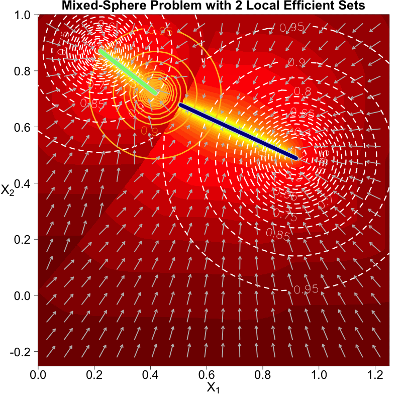
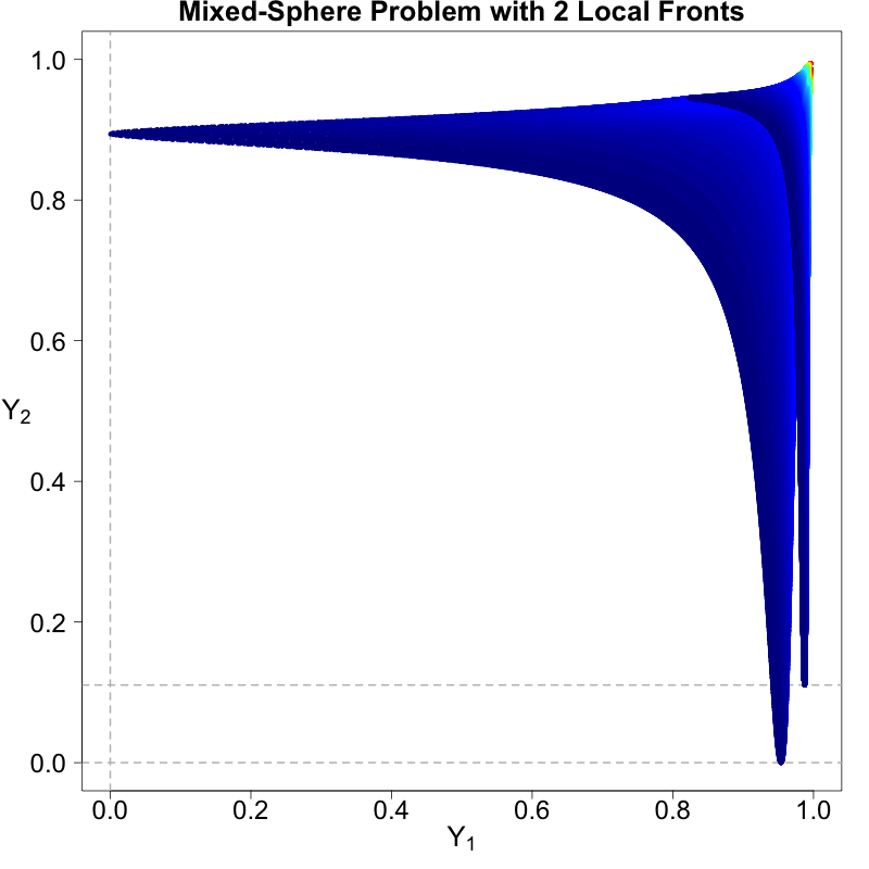
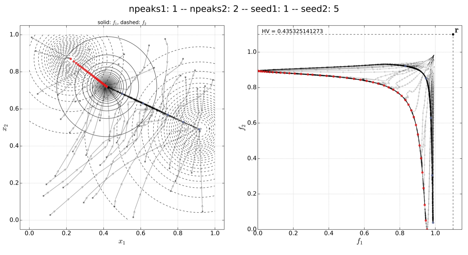
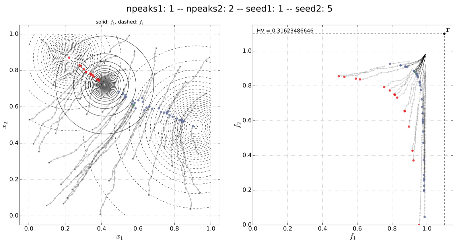
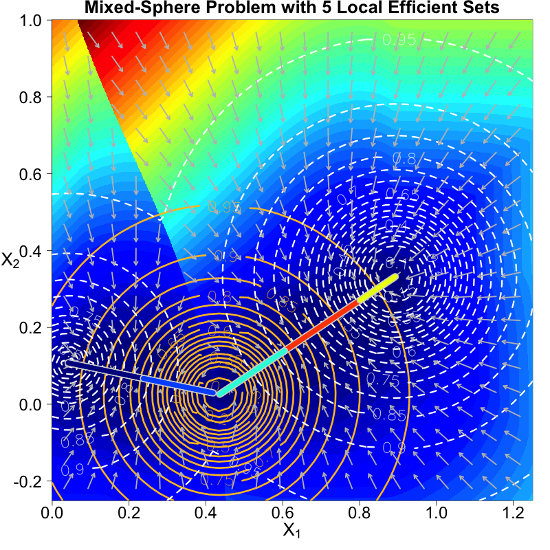
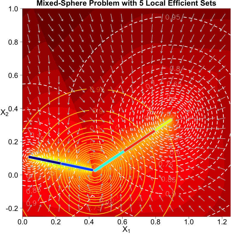
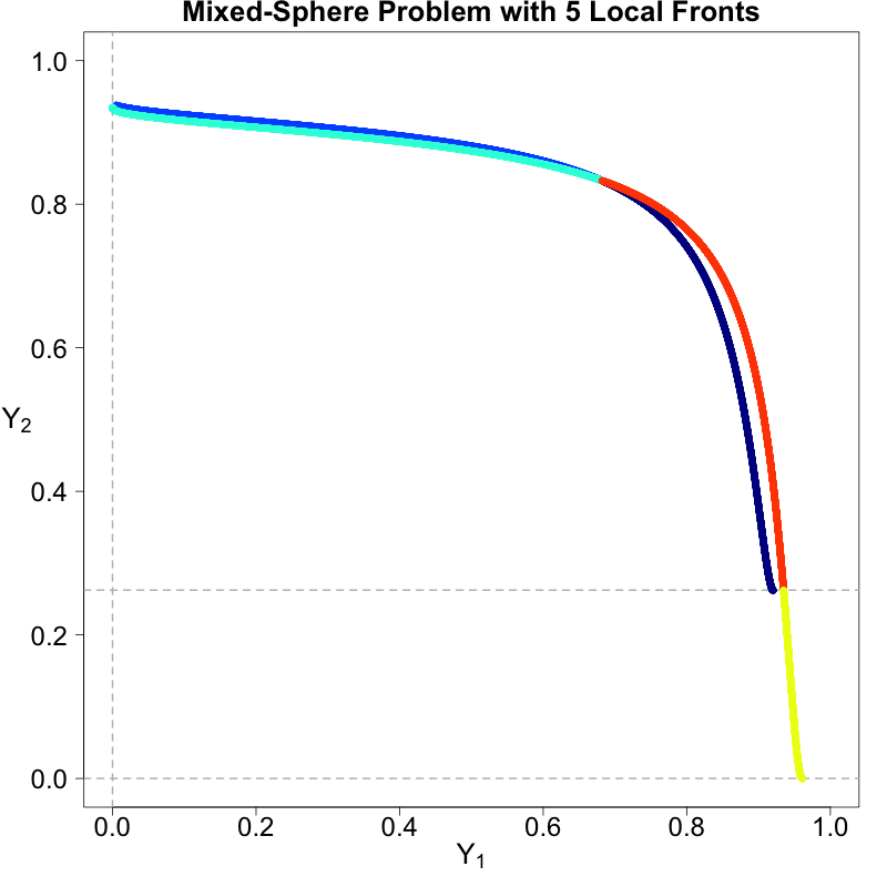
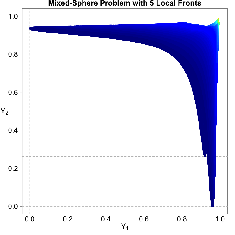
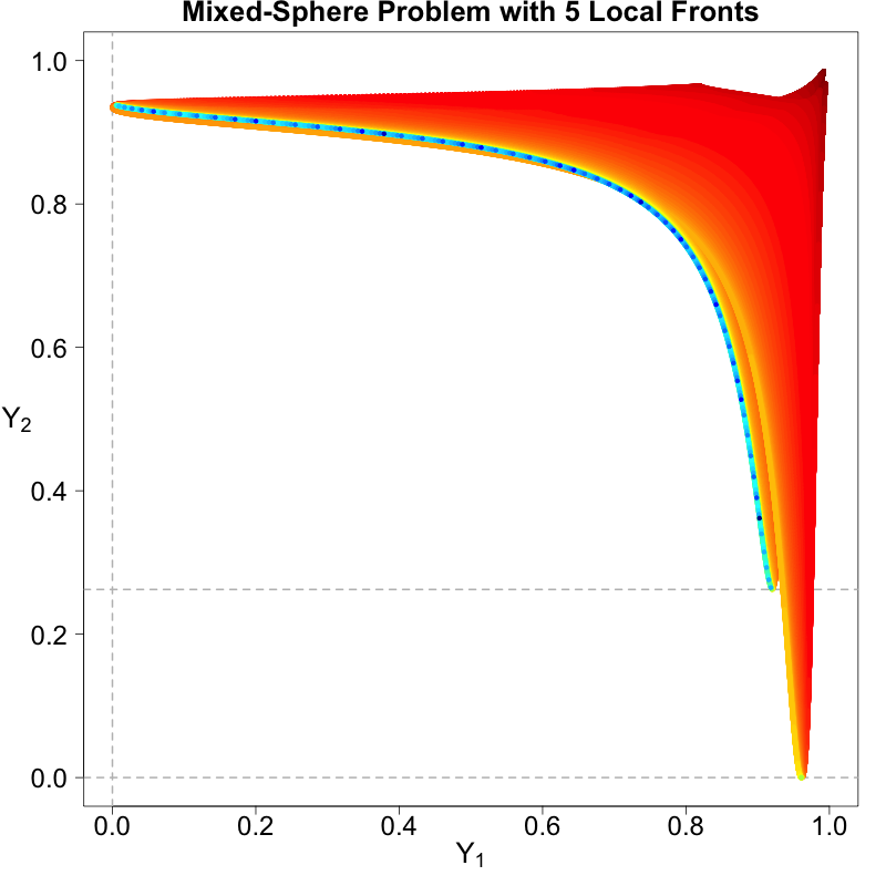
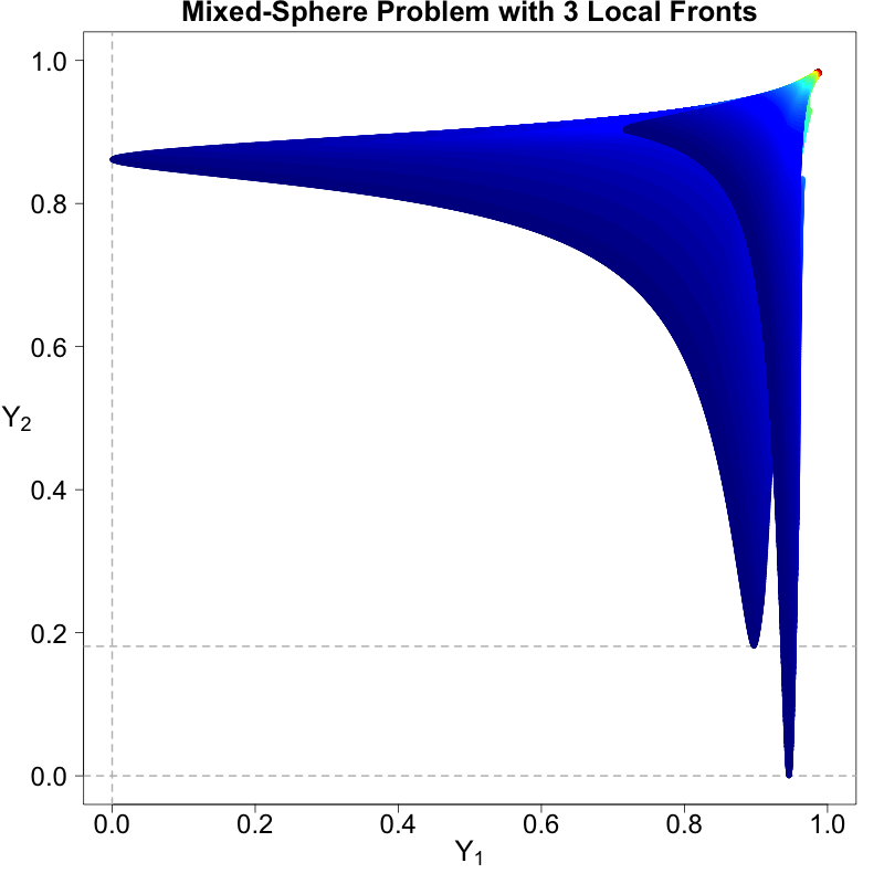
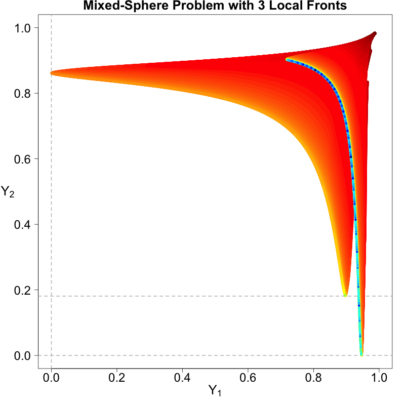
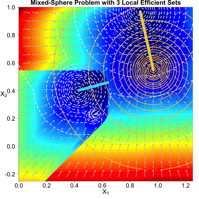
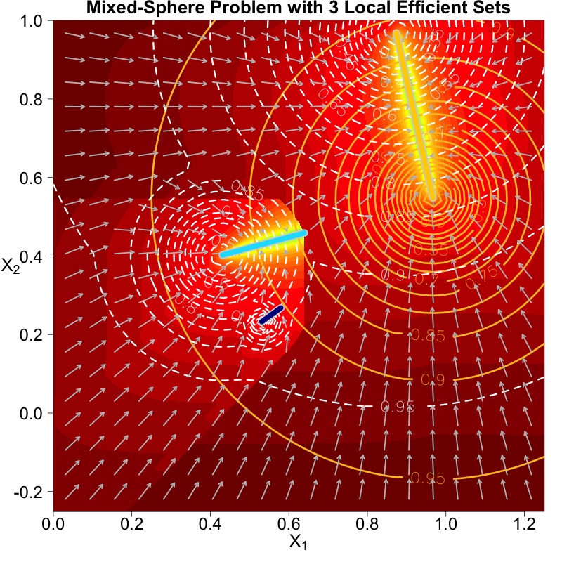
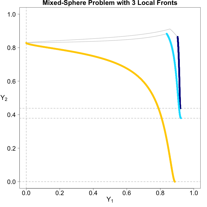
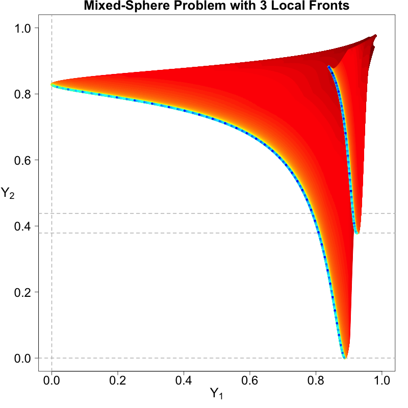
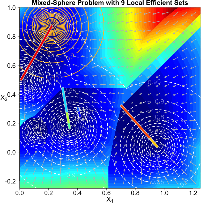
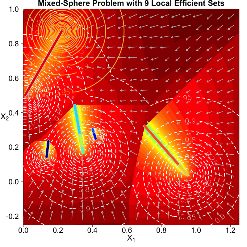
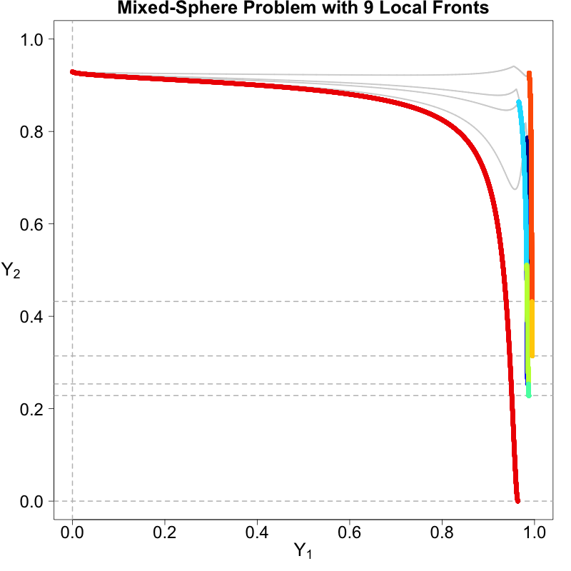
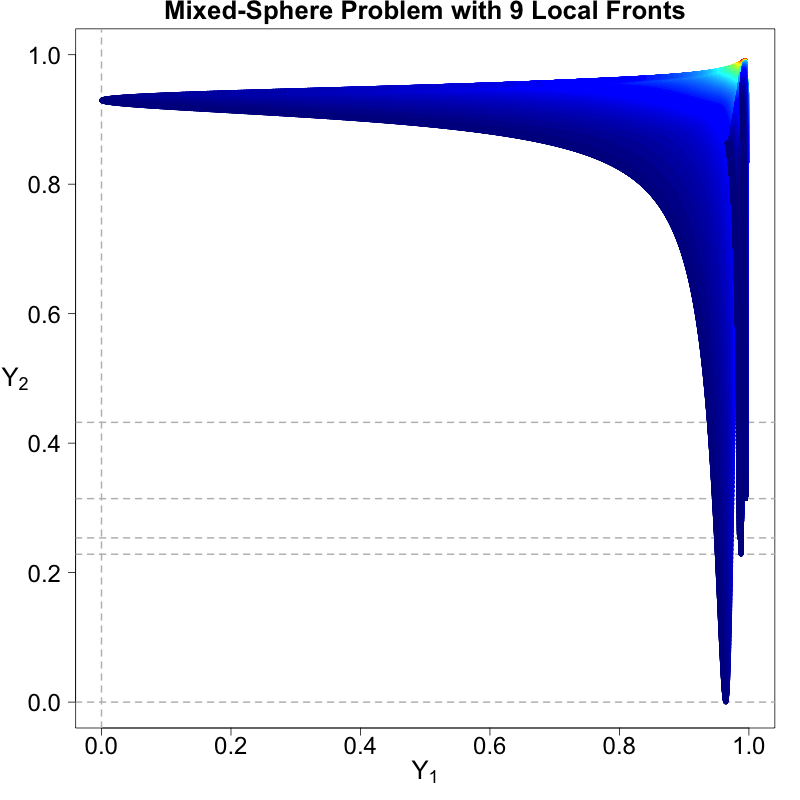
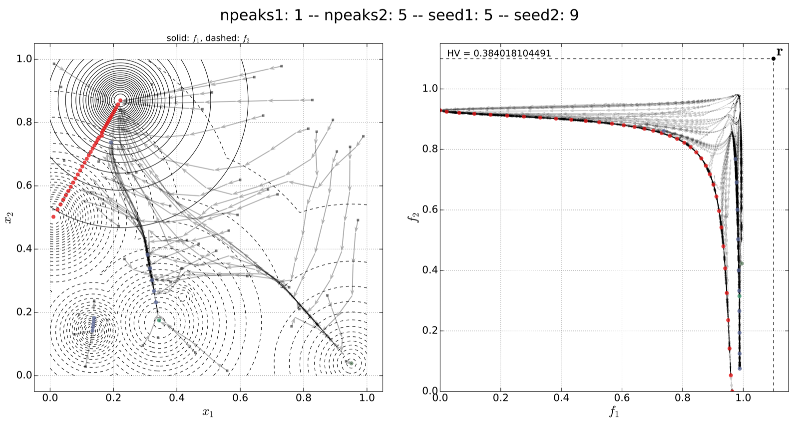
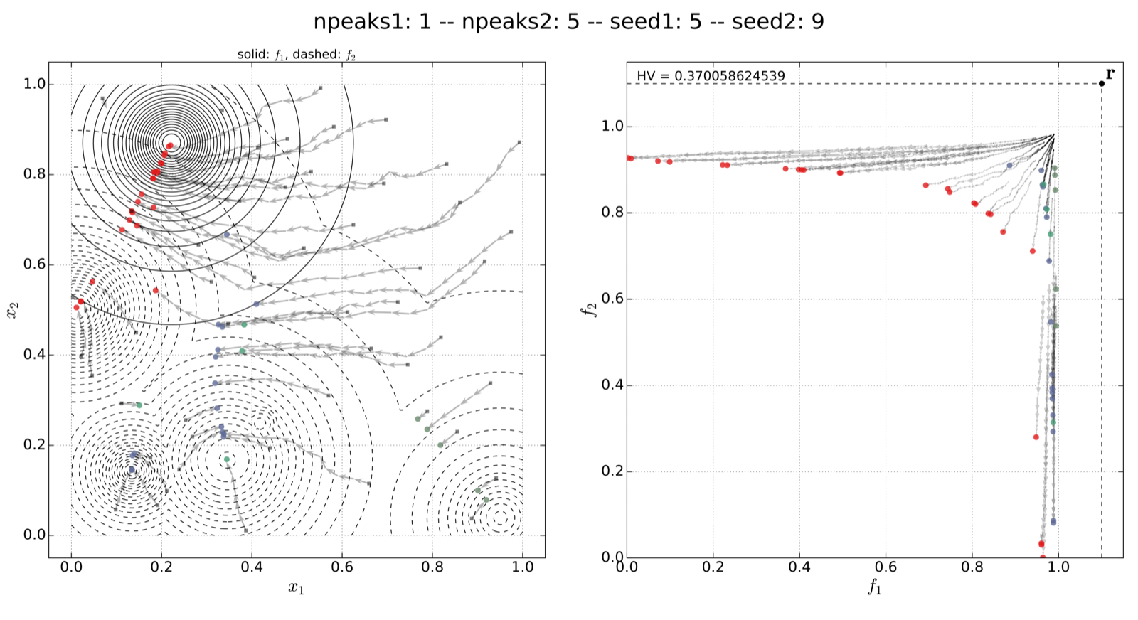
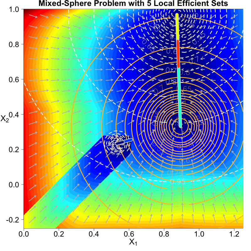
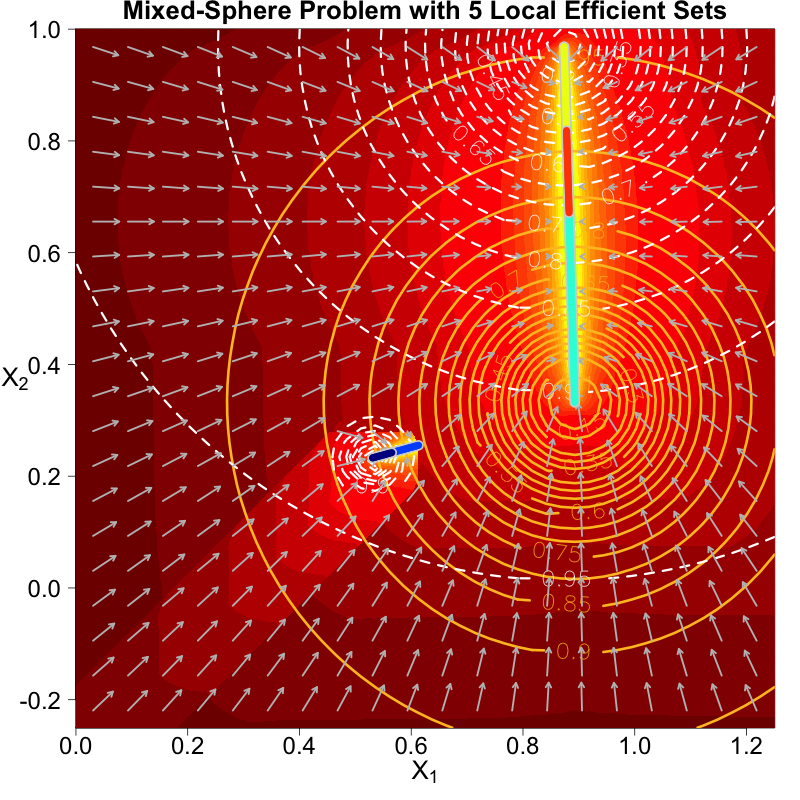
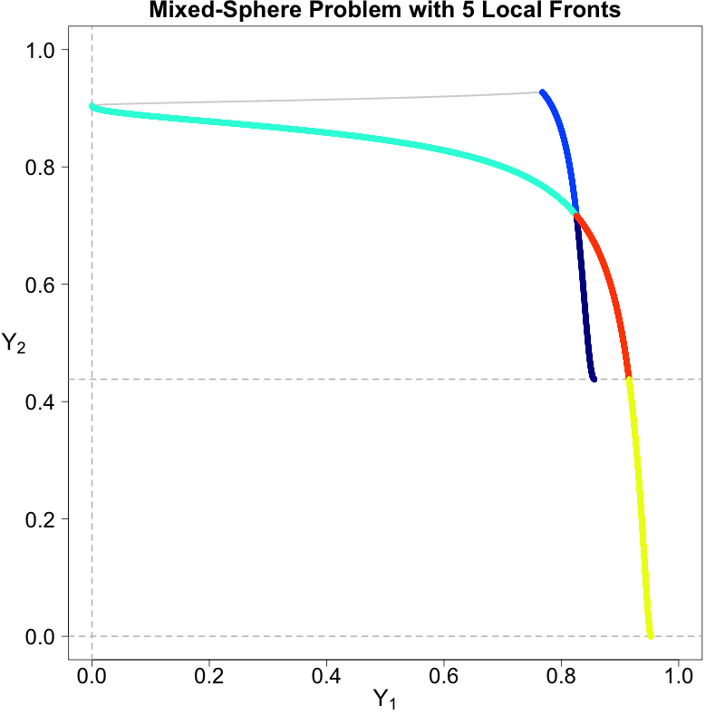
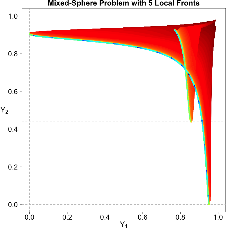
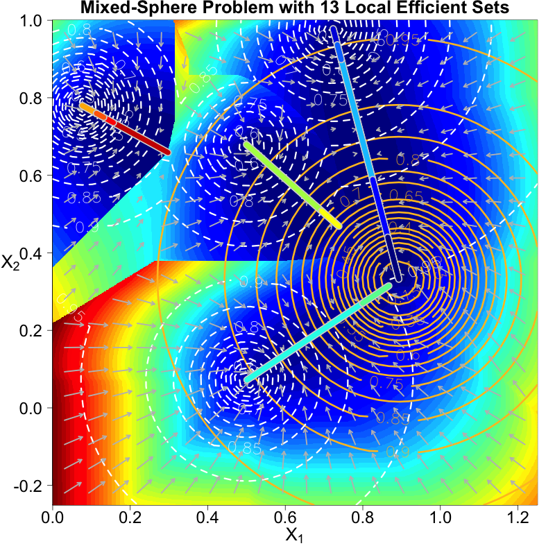
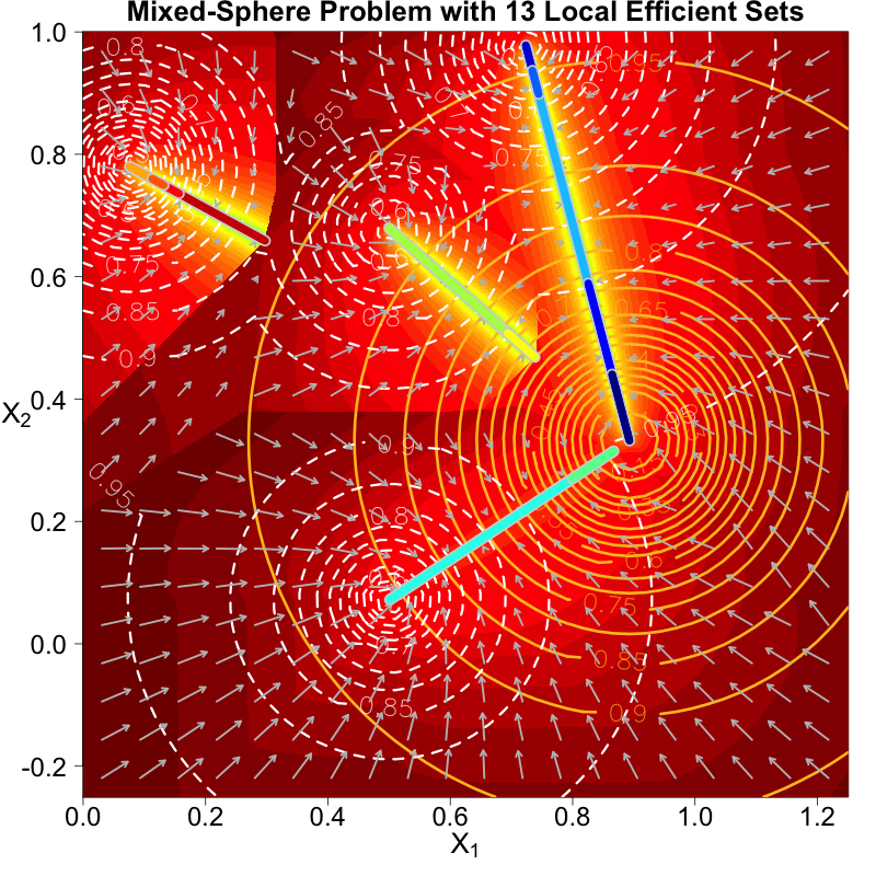
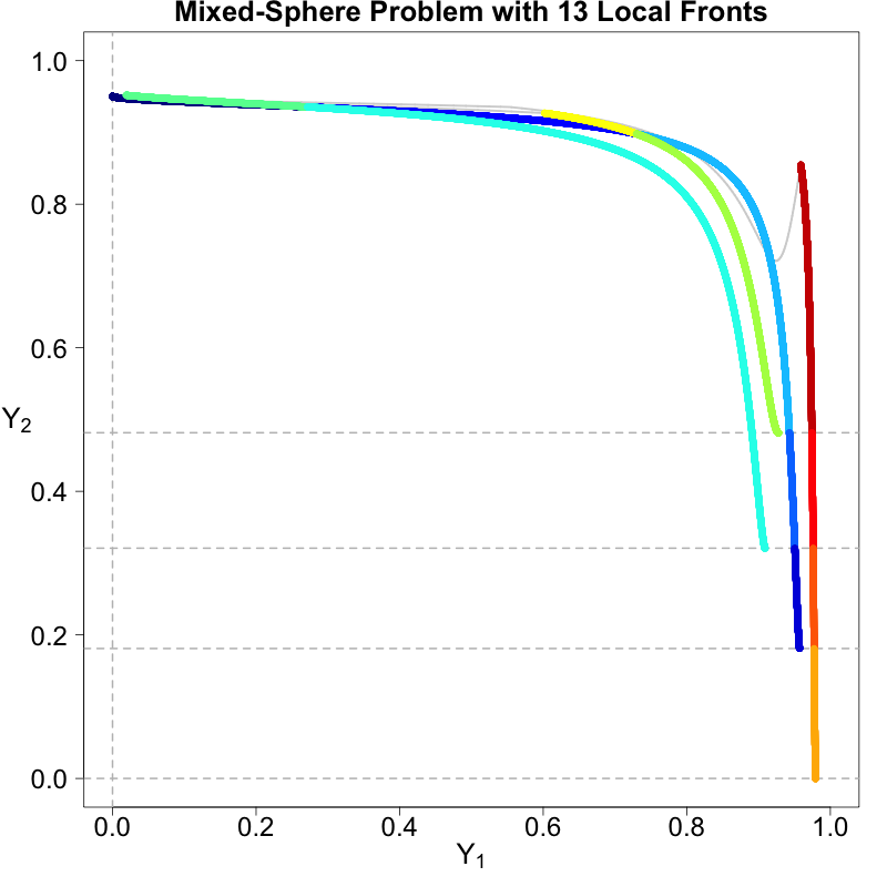
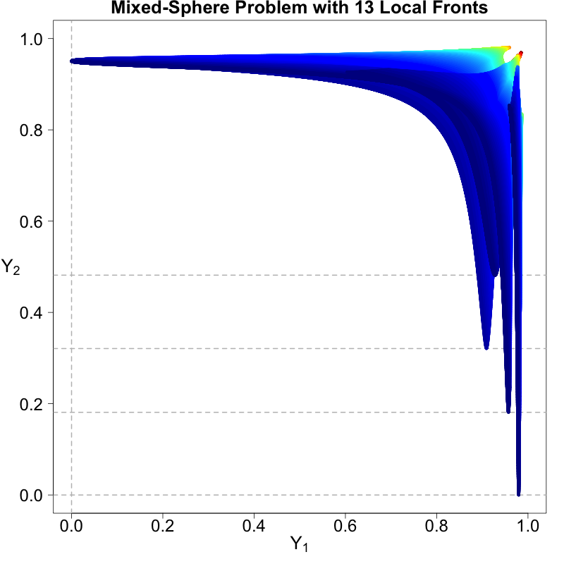
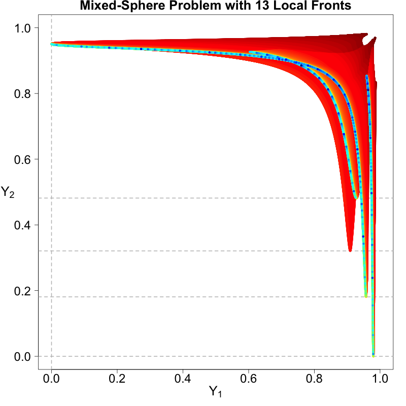
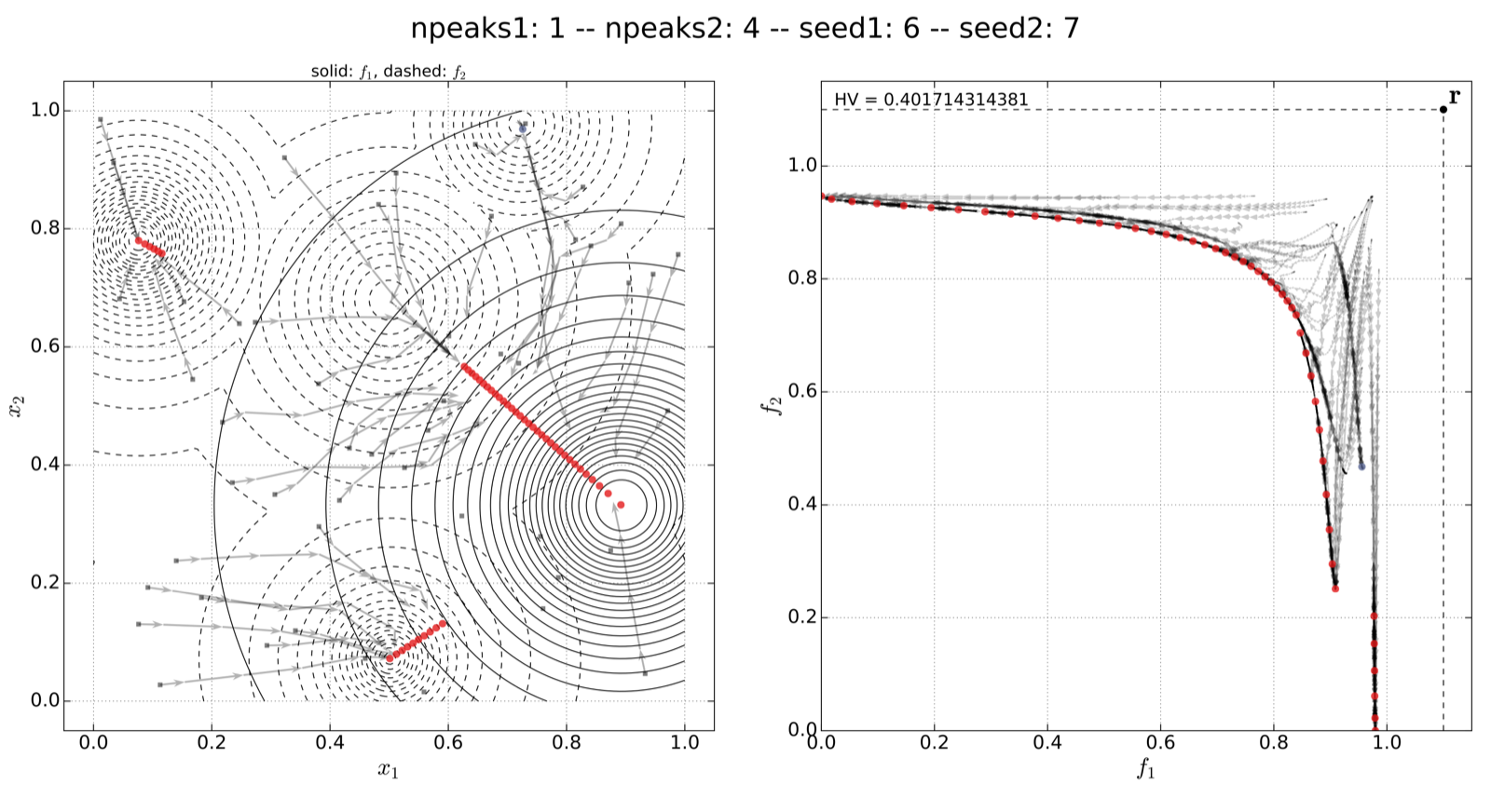
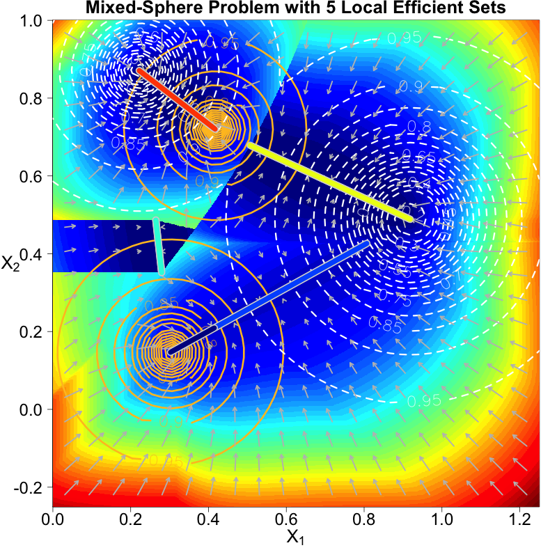
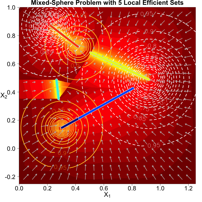
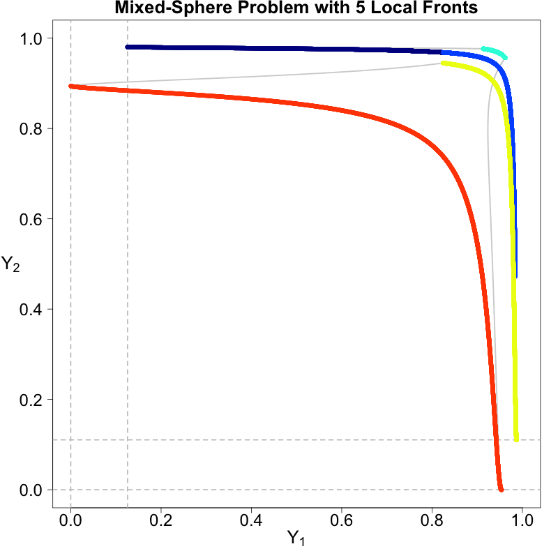
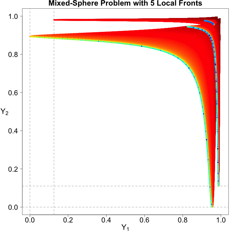
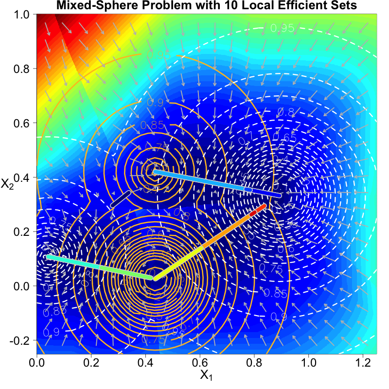
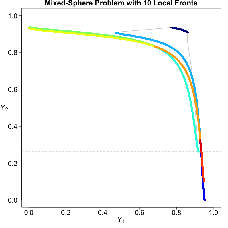
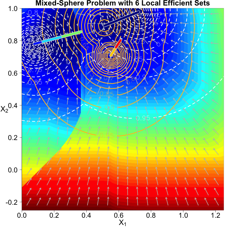
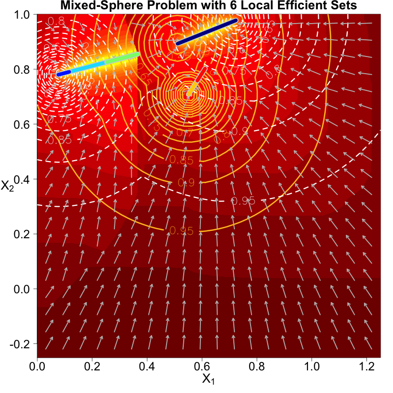
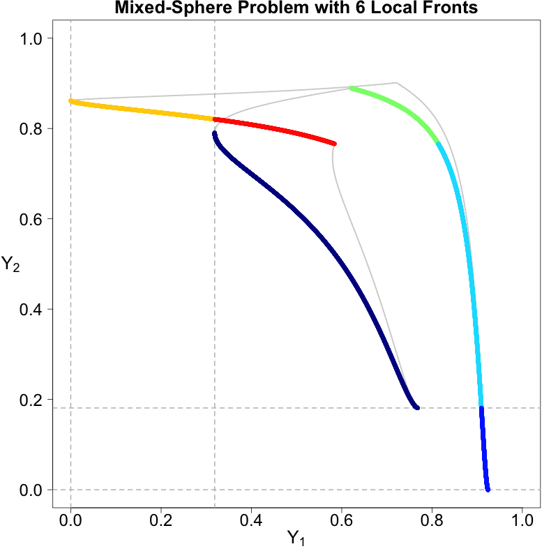
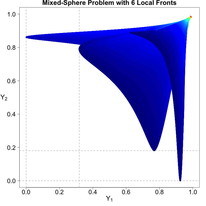
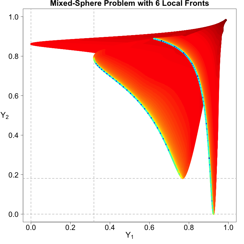
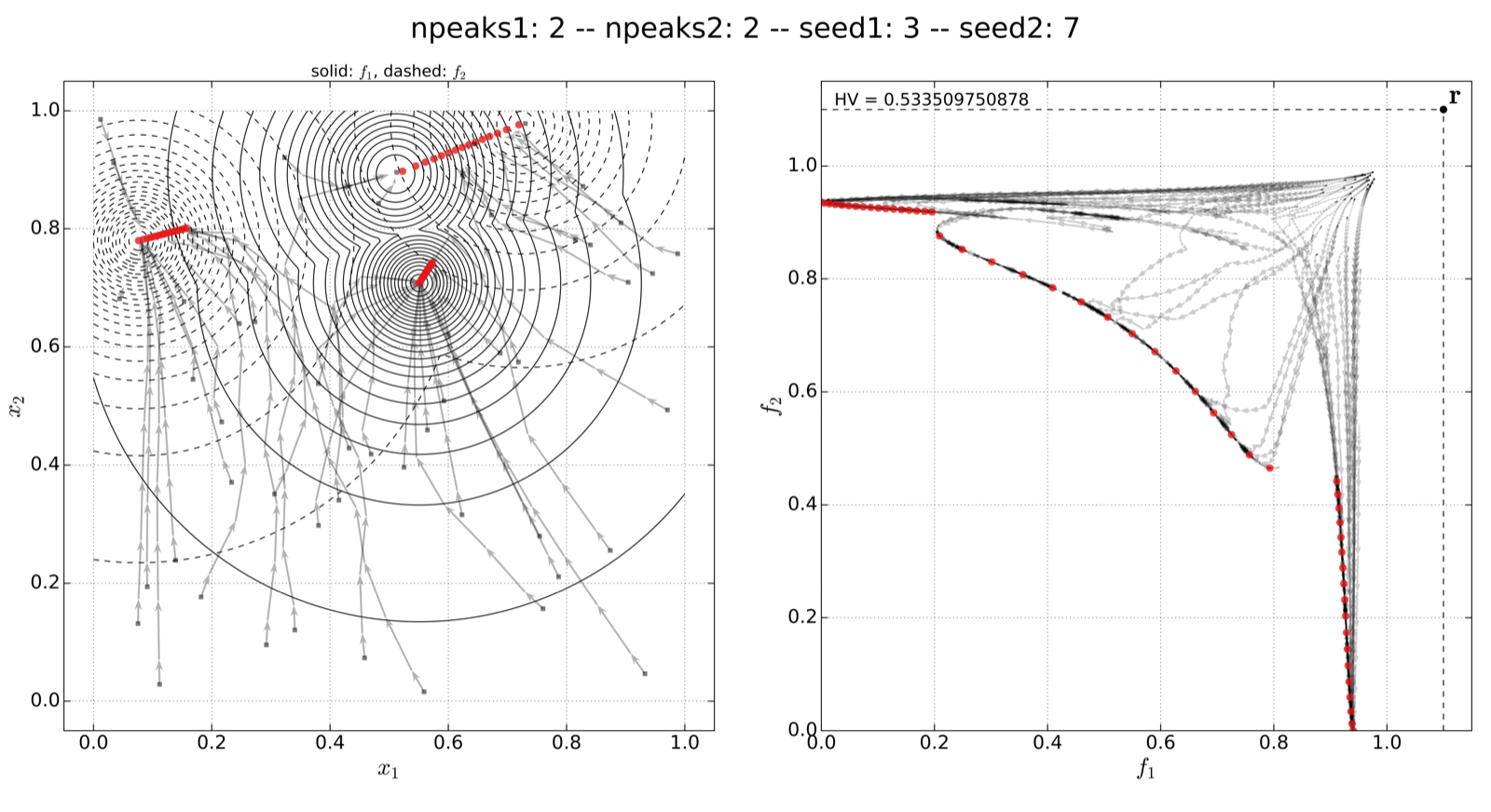
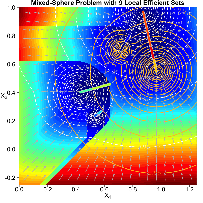
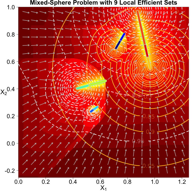
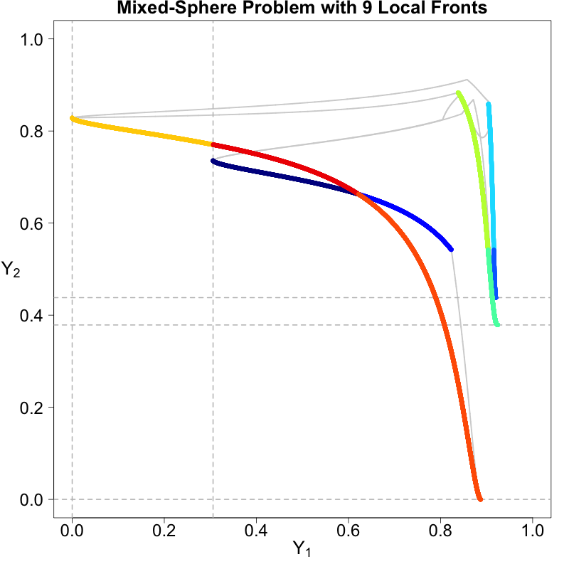
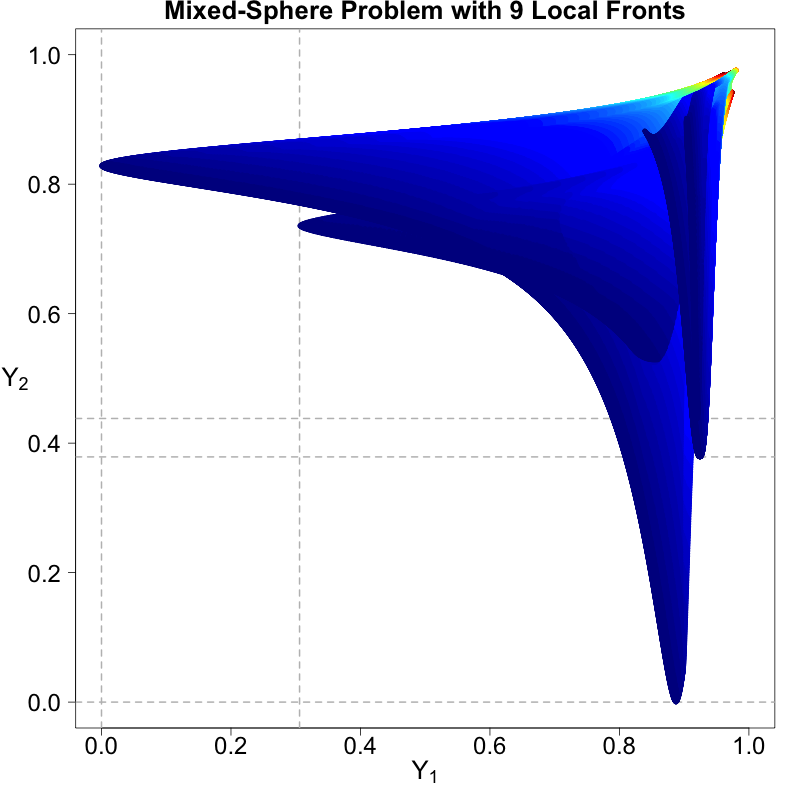
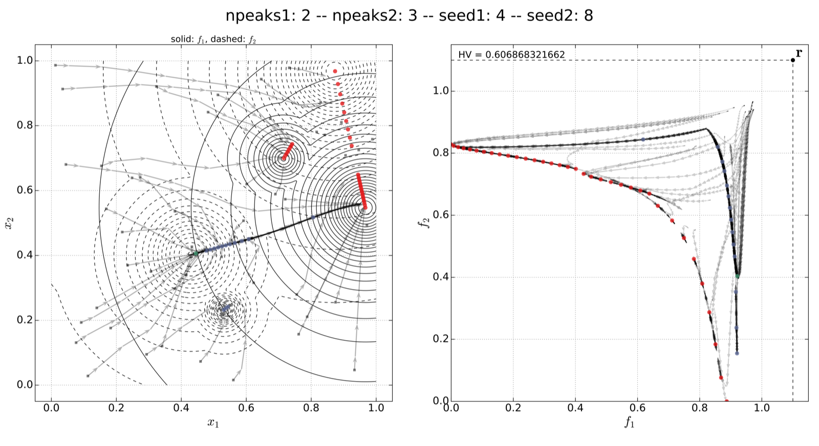
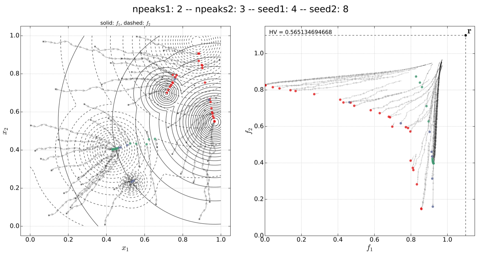
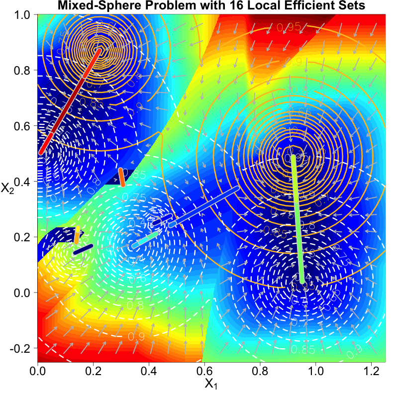
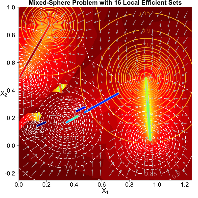
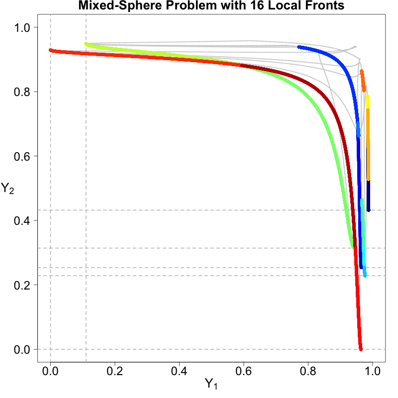
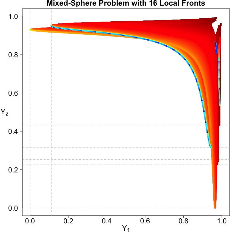
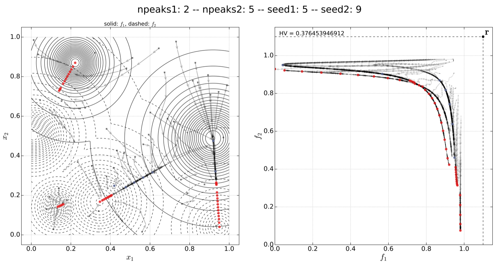
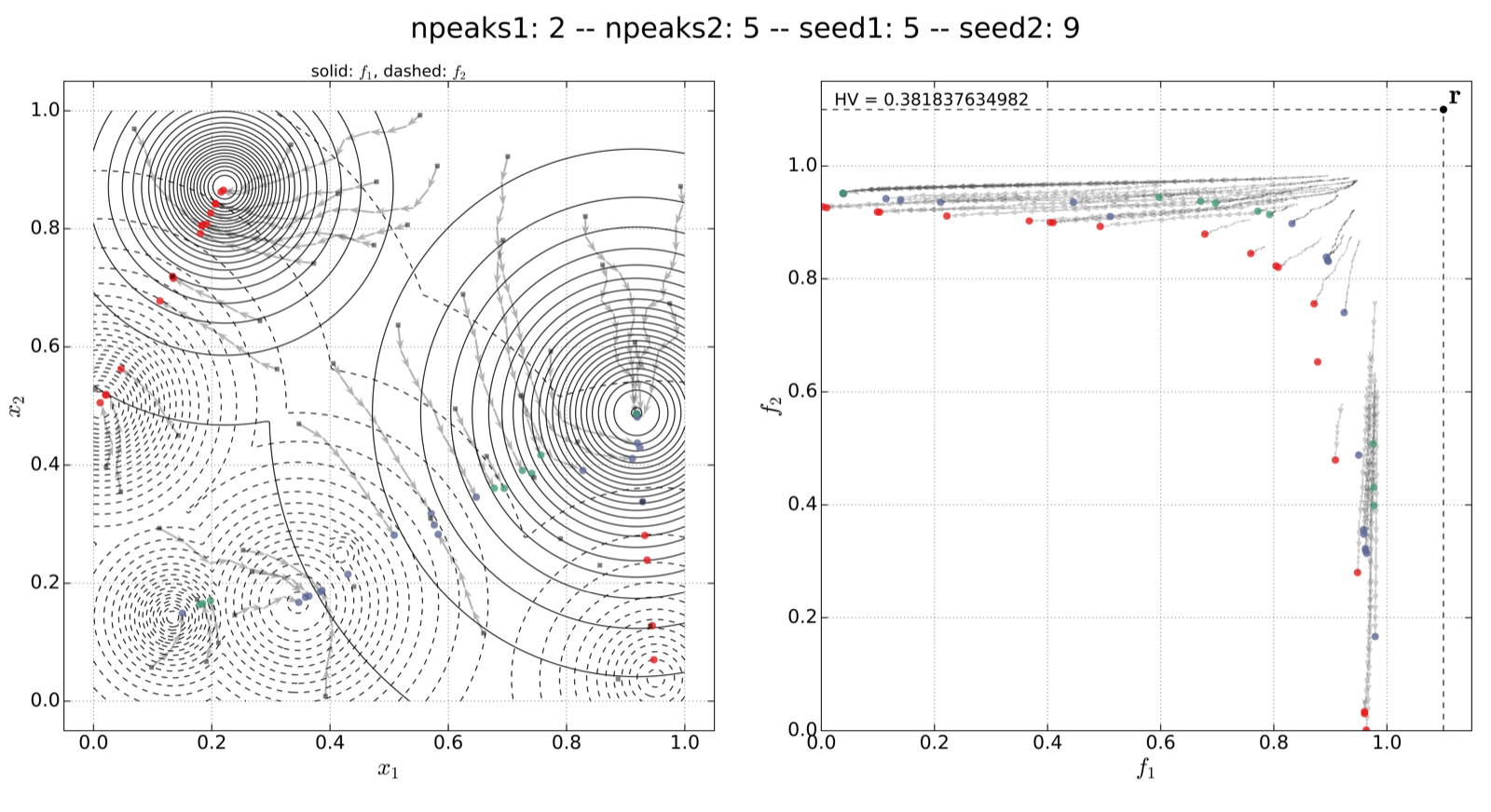
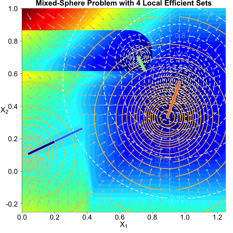
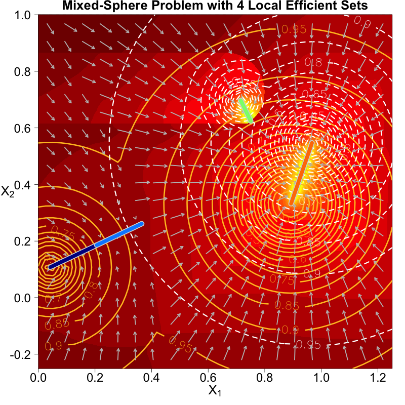
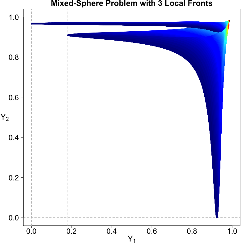
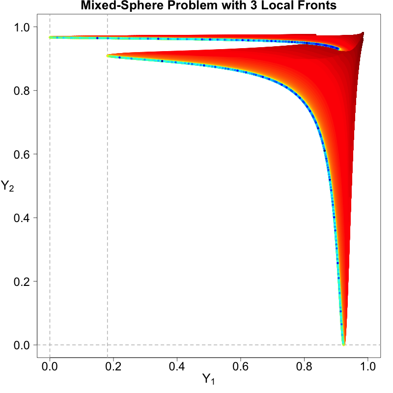
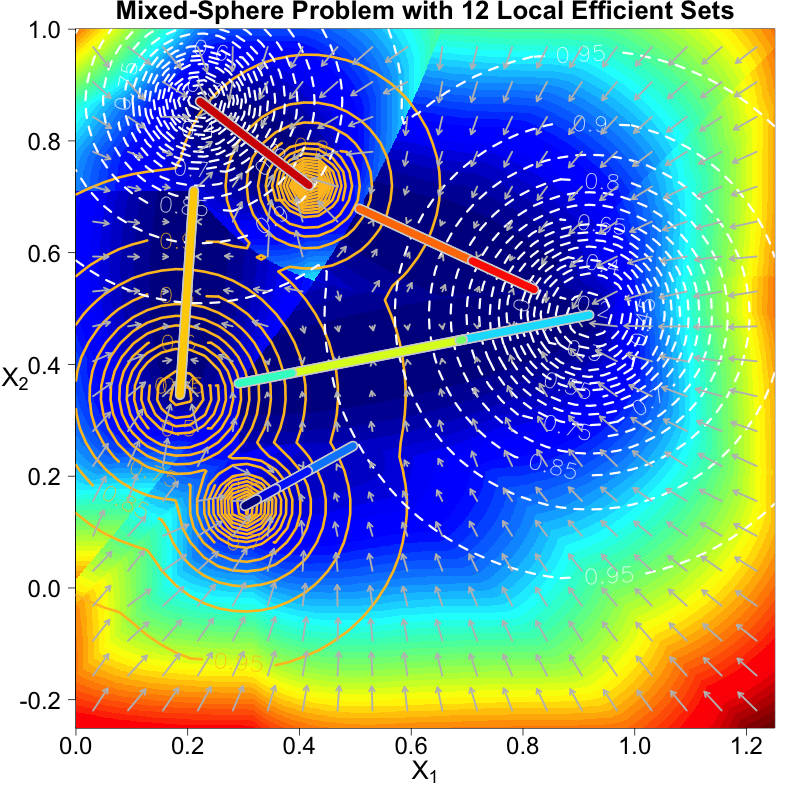
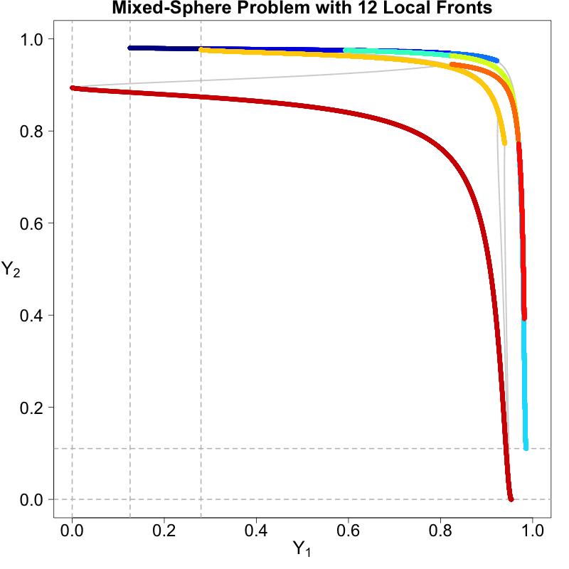
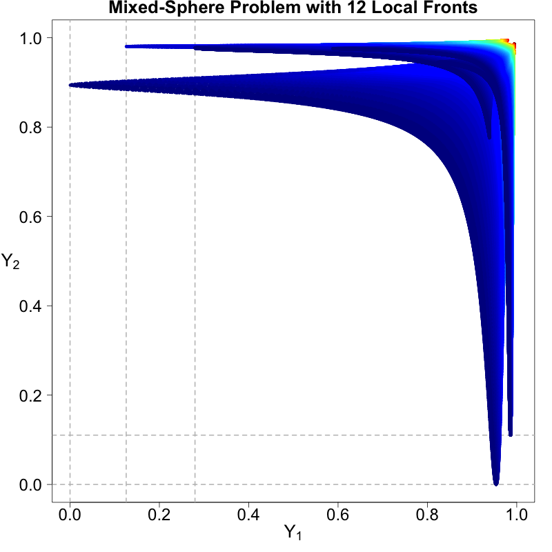
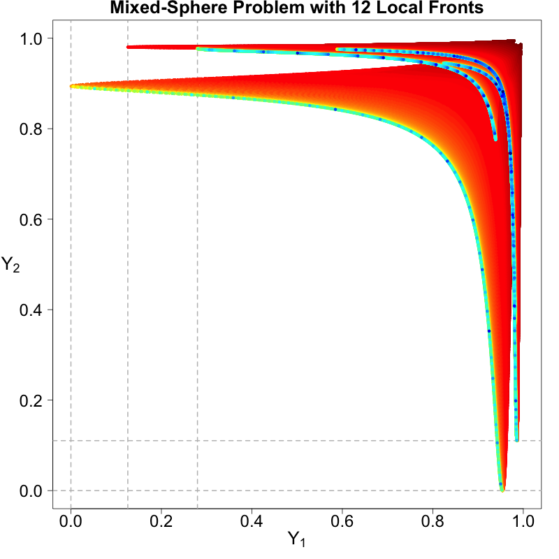
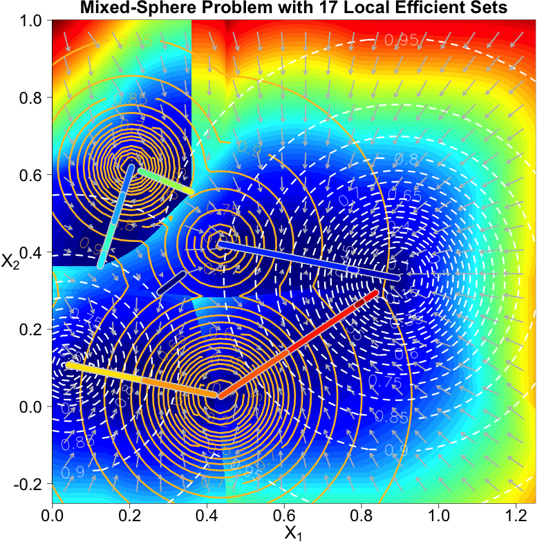
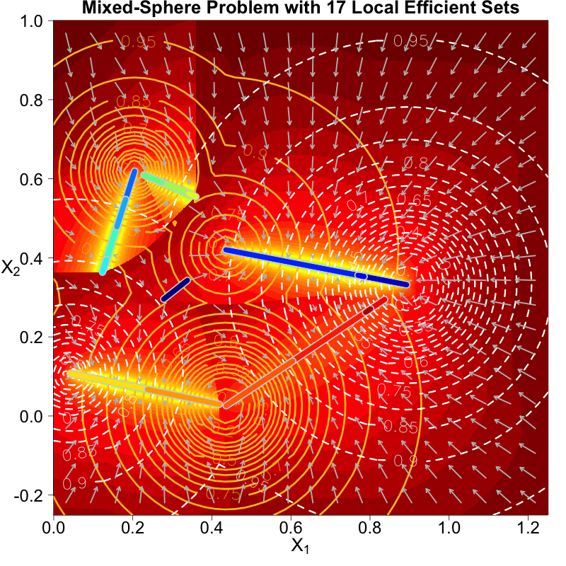
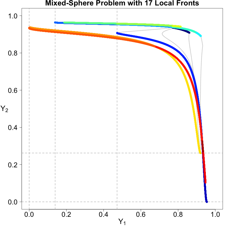
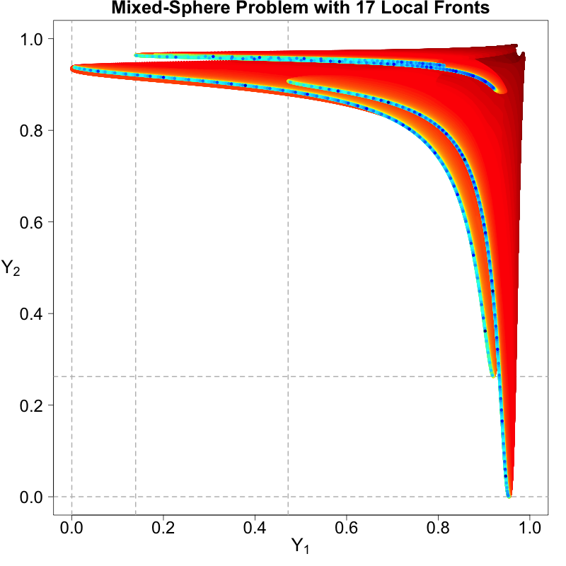
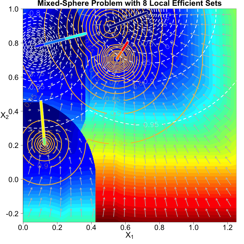
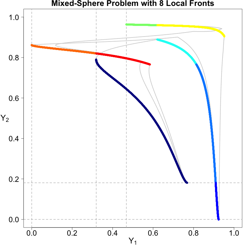
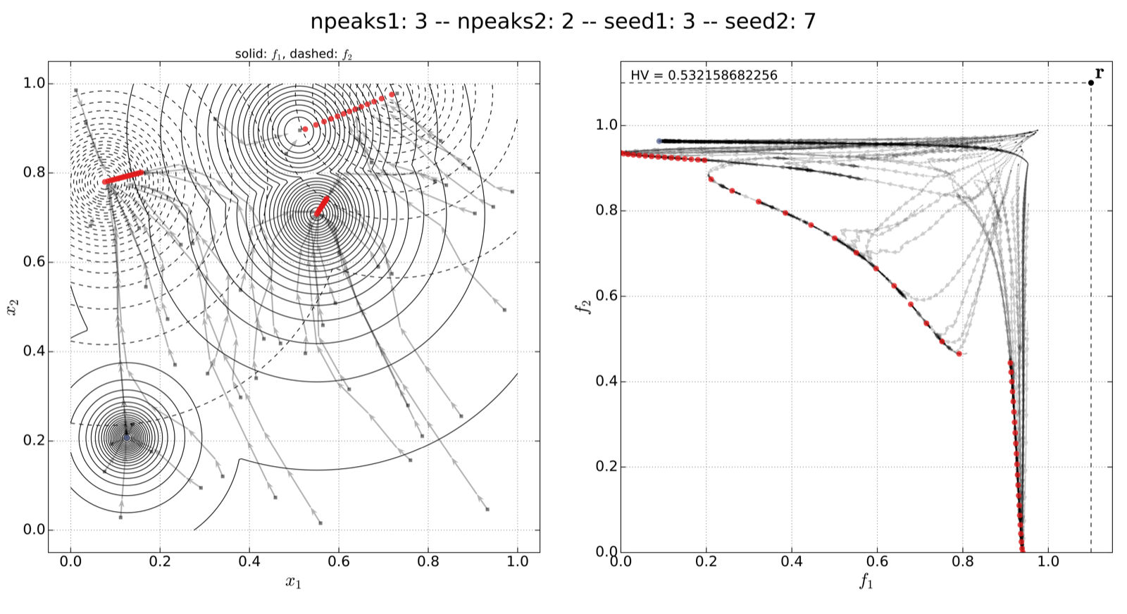
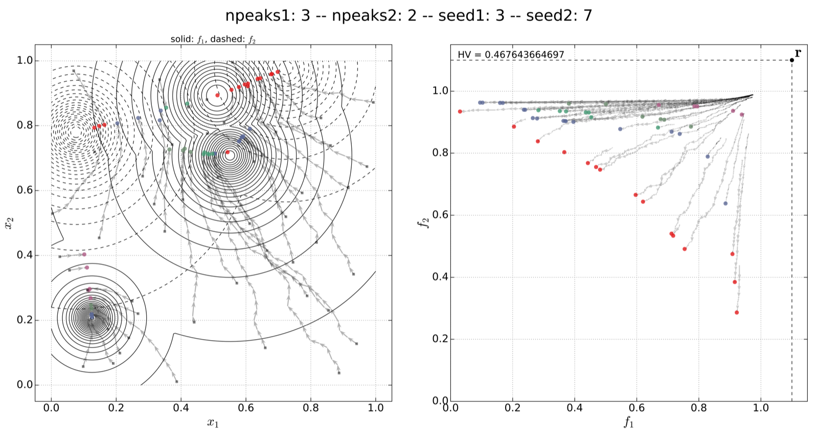
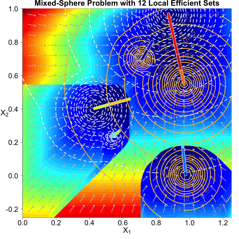
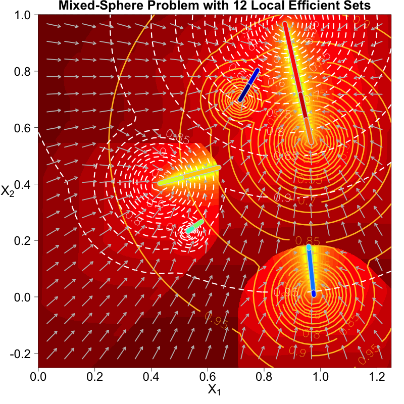
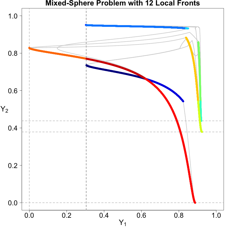
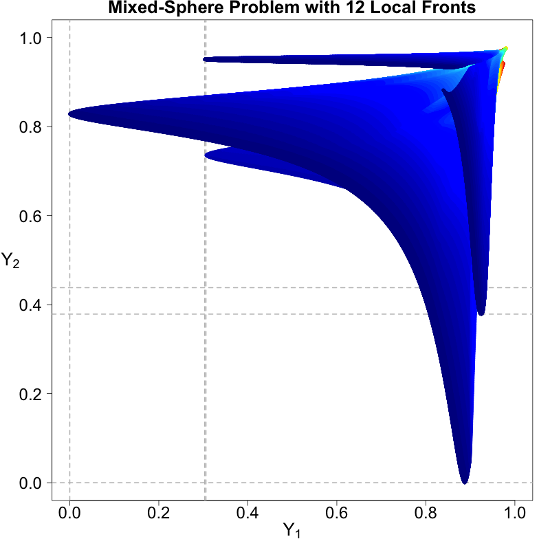
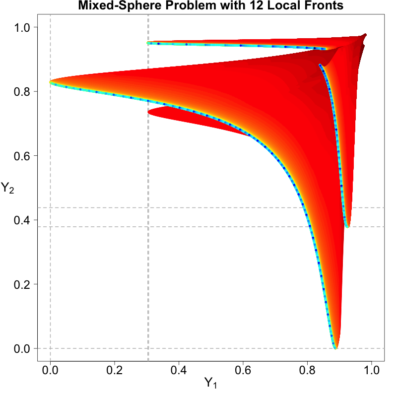
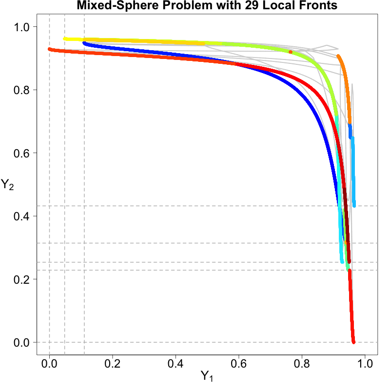
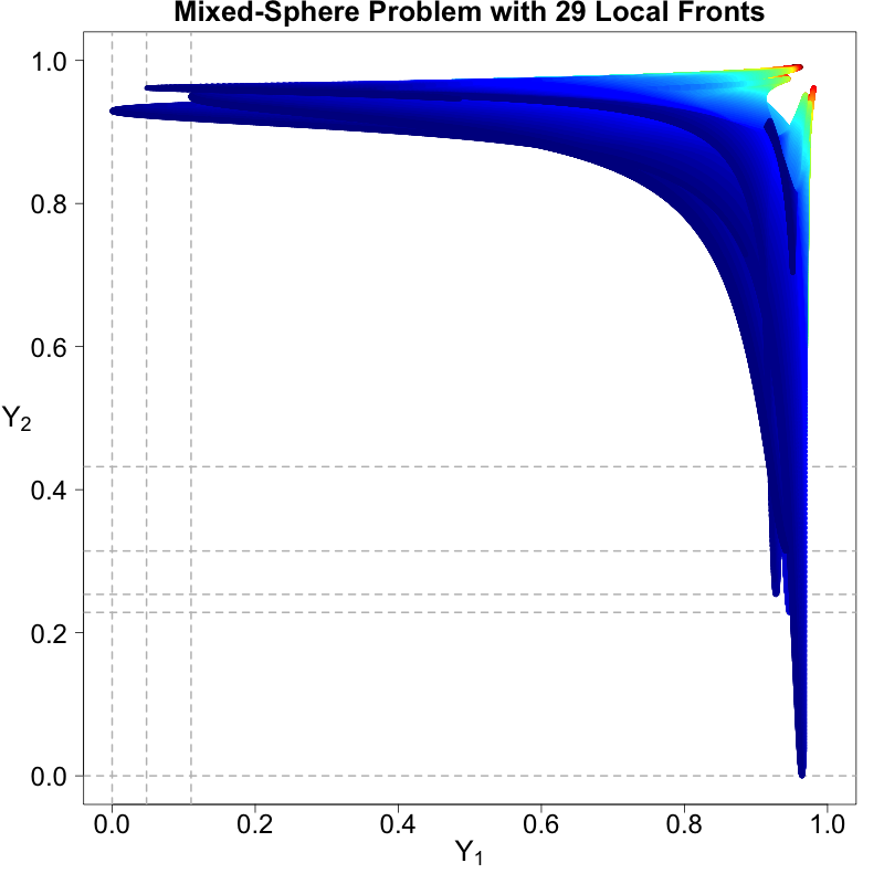
The table below provides information on the 40 problem instances from our bi-objective mixed-sphere / mixed-ellipsoid benchmark. Each of the problems is a combination of two single-objectives problems, created using the MPM2 generator (Wessing, 2015). Those problems can for instance be created using the R-package smoof 1.5 (Bossek, 2017) or the python package optproblems 0.9 (Wessing, 2016). The columns of the table describe the following:
- ID of the benchmark problem (a value between 1 and 40)
- Problem Setup, i.e., the parameters for configuring each of the two objectives per instance:
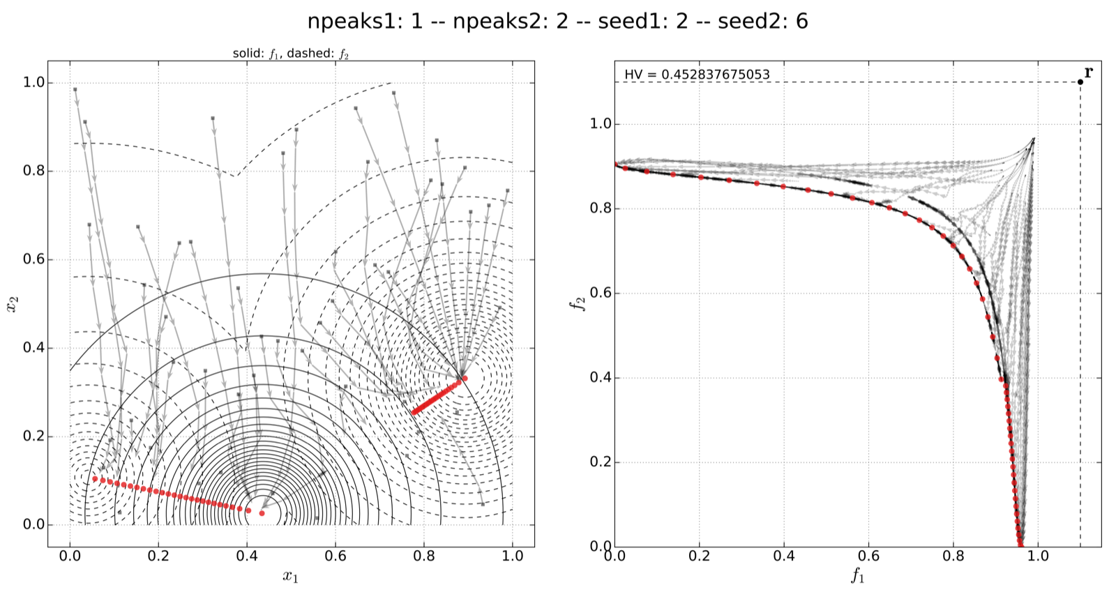
- Shape of the Peaks:
Shape of the contour lines of the peaks (either "ellipse" or "sphere"). - Rotate Peaks:
Should the peak shapes be rotated (TRUE / FALSE)? This parameter is only useful, if the peak shape is "ellipse". - Problem Dimension:
Number of input input parameters (i.e., dimensions of the search space). - Topology:
How should the peaks be aligned per objective? Possible values are "random" or "funnel". - # Peaks:
The number of peaks for each of the two objectives. - Seed:
The seed that was used for generating each of the single-objective functions
- Shape of the Peaks:
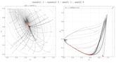
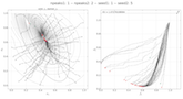
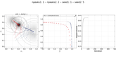
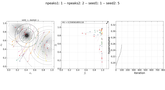
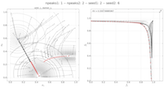
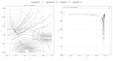
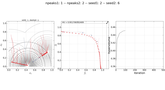
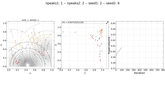
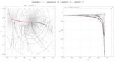
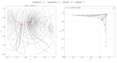
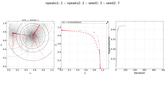
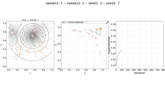
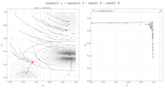
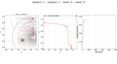
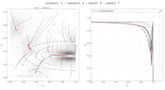
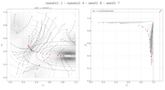
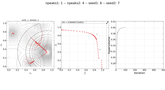
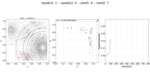
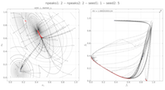
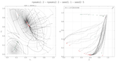
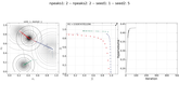
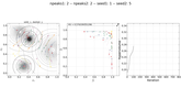
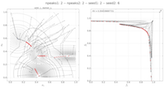
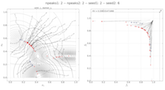
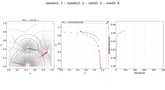
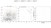
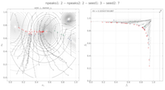
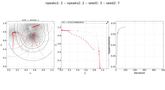
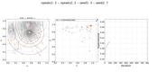
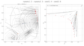
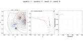
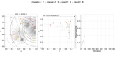
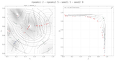
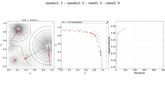
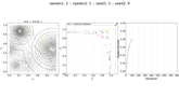
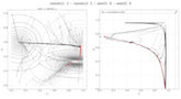
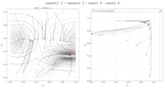
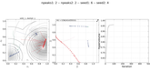
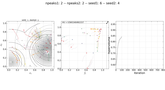
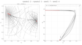
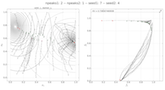
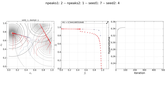
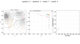
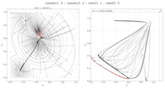
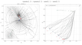
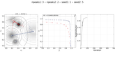
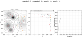
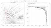
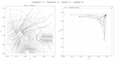
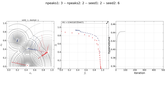
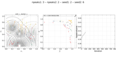
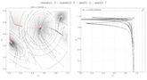
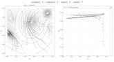
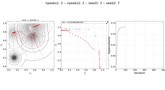
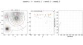
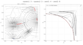
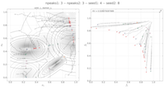
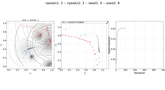
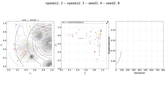
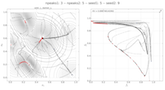
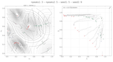
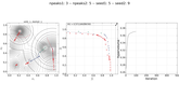
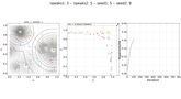
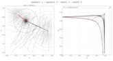
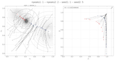
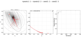
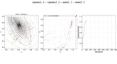
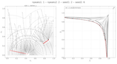
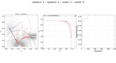
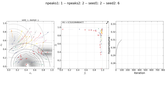
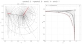
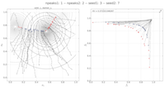
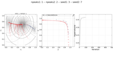
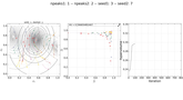
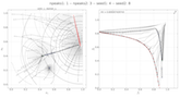
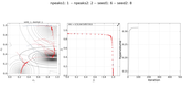
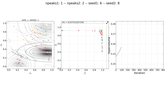
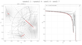
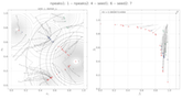
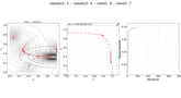
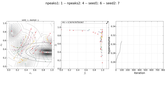
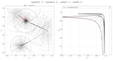
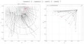
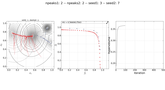
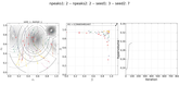
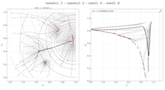
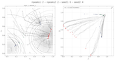
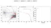
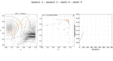
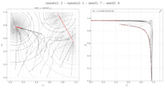
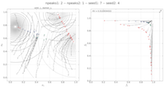
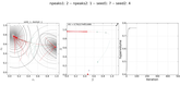
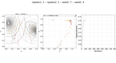
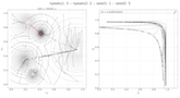
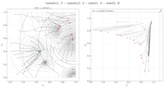
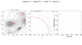
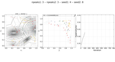
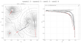
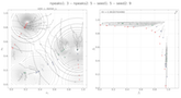
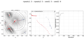
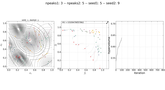
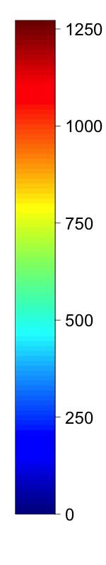
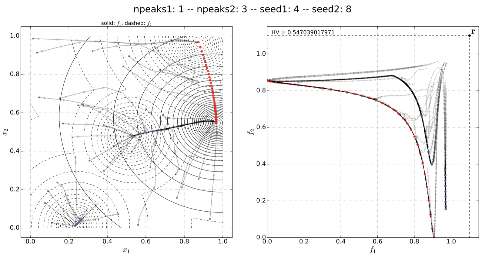
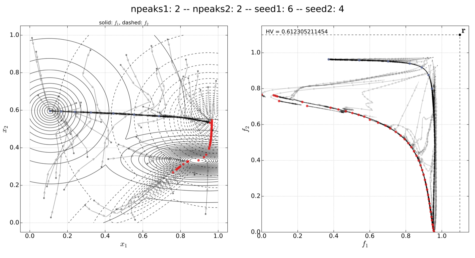
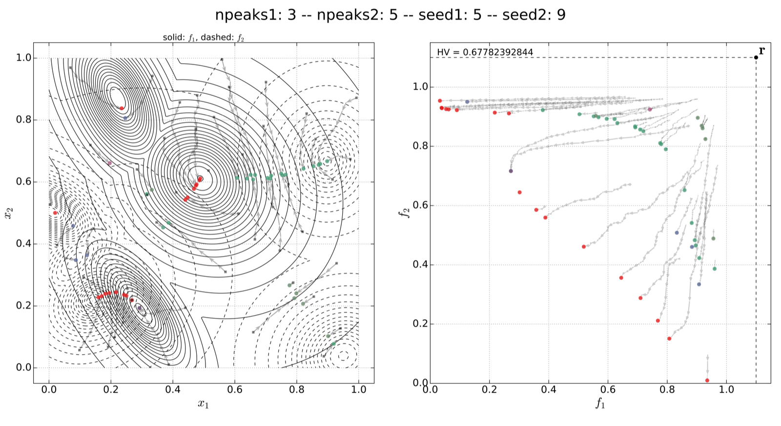
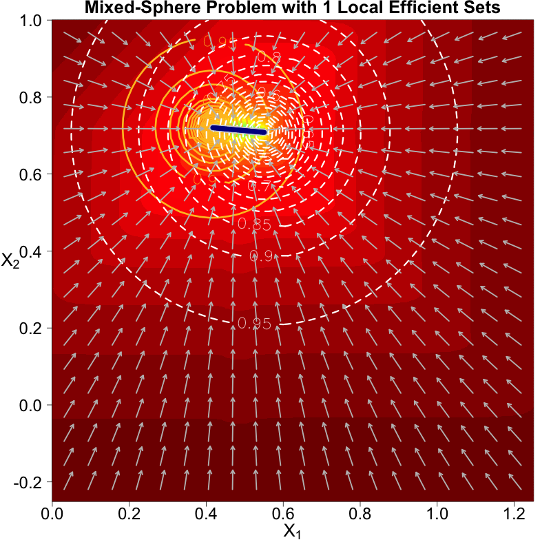
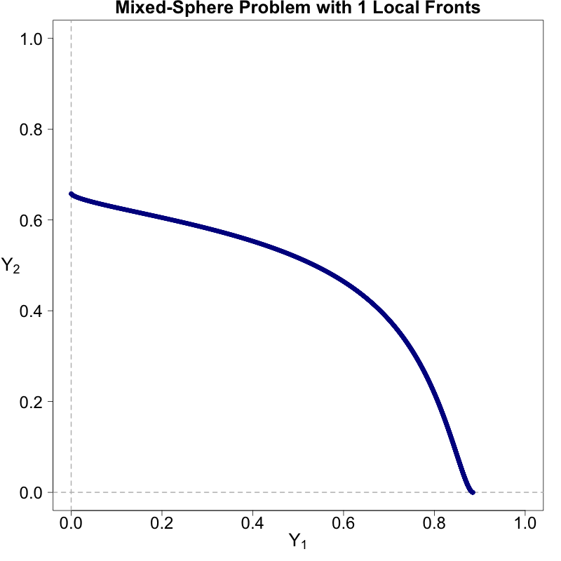
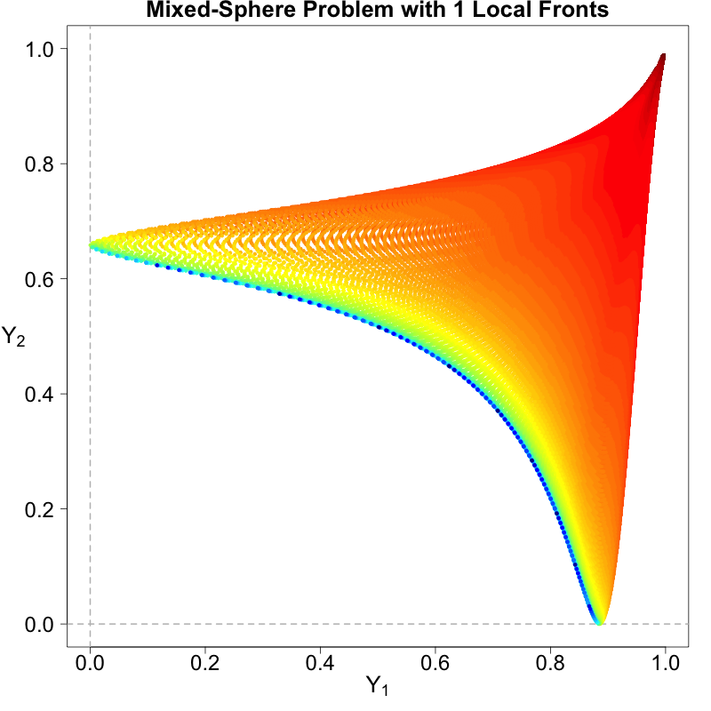
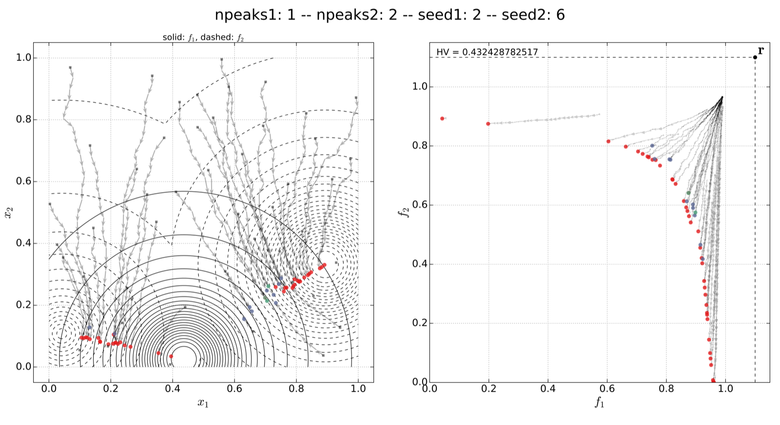
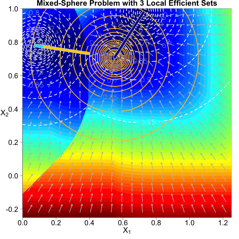
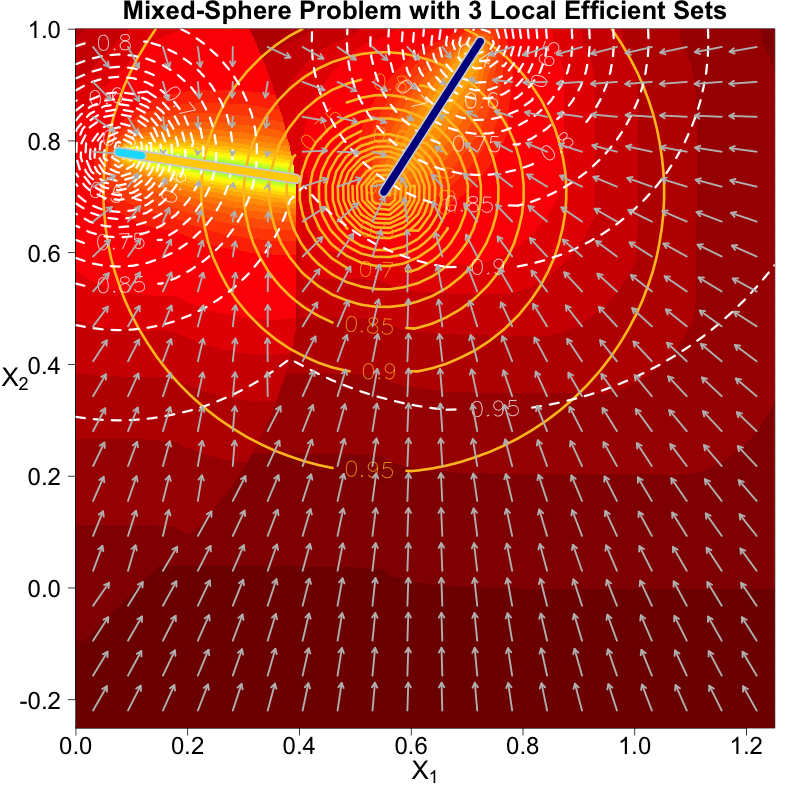
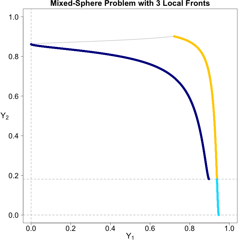
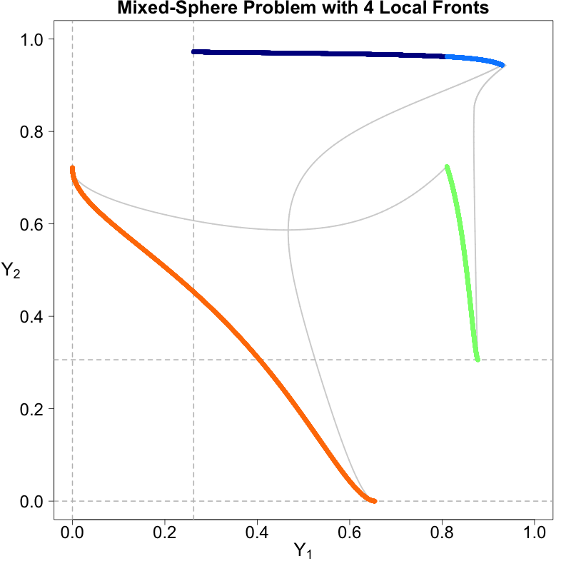
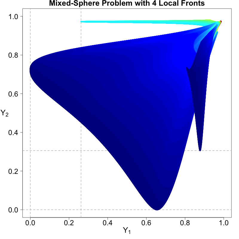
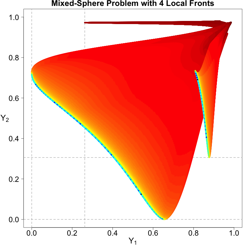
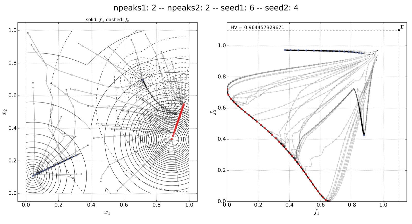
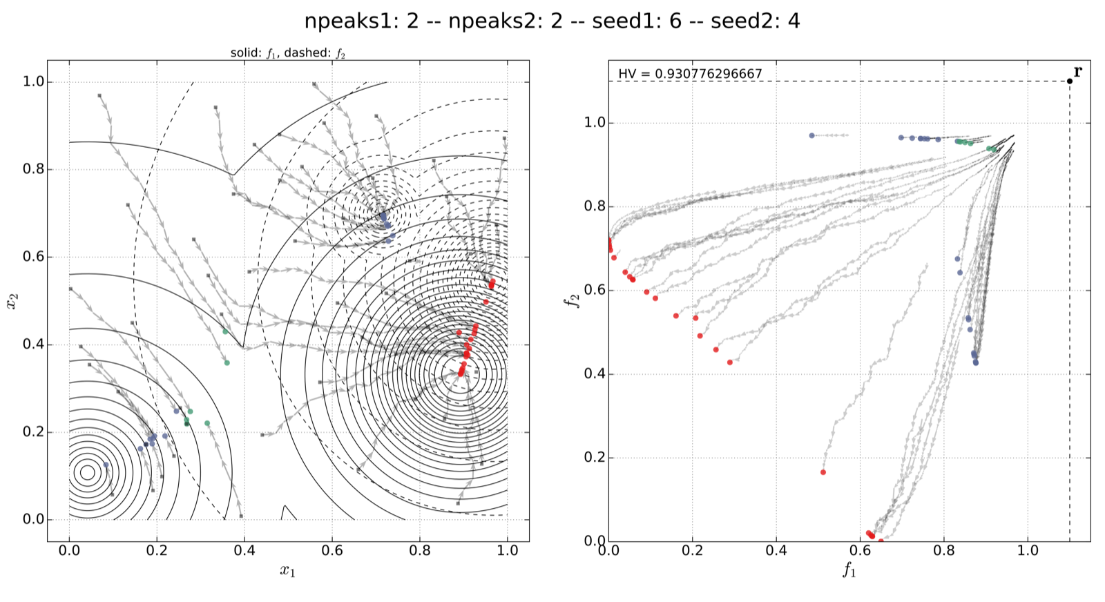
- Visual Results:
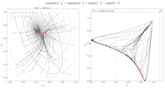
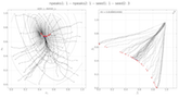
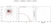
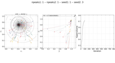
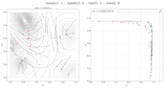
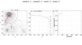
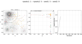
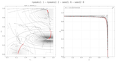
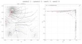
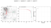
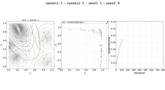
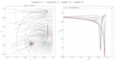
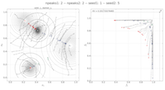
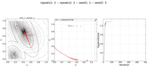
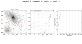
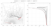
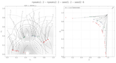
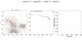
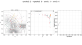
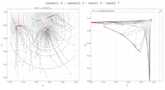
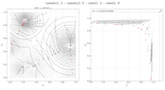
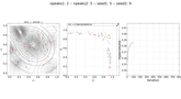
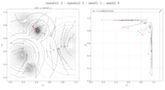
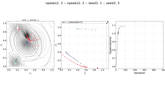
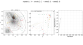
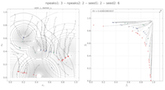
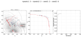
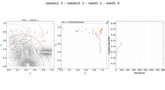
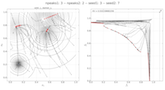
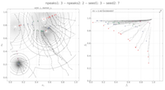
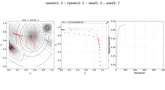
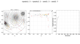
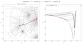
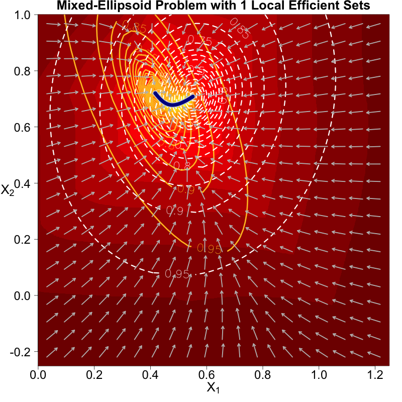
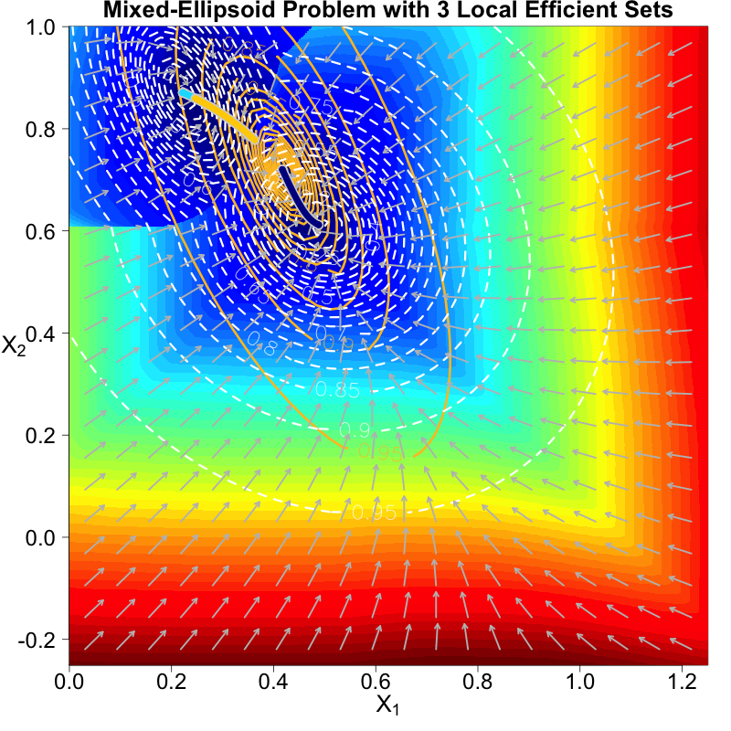
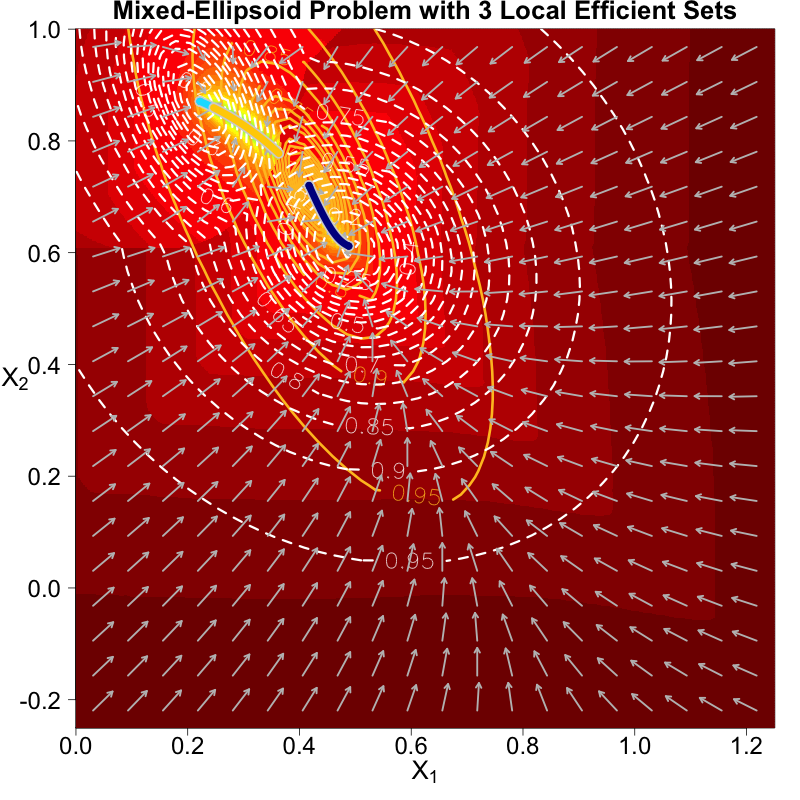
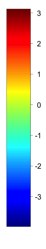
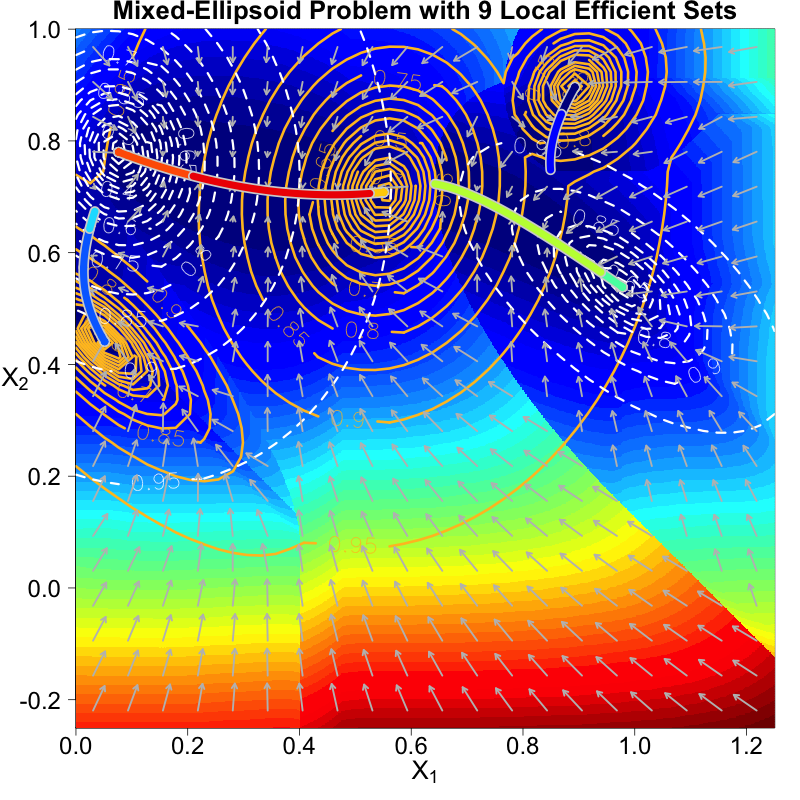
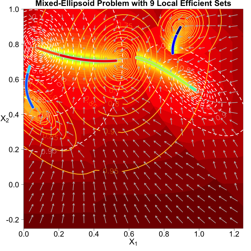
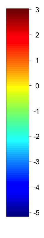
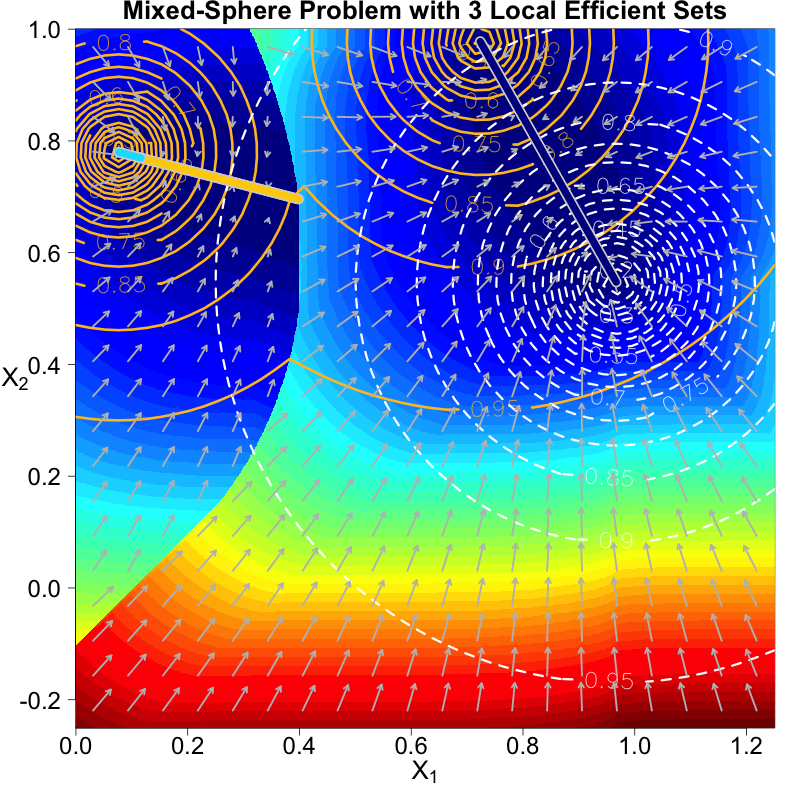
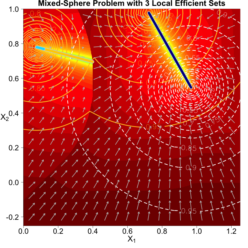
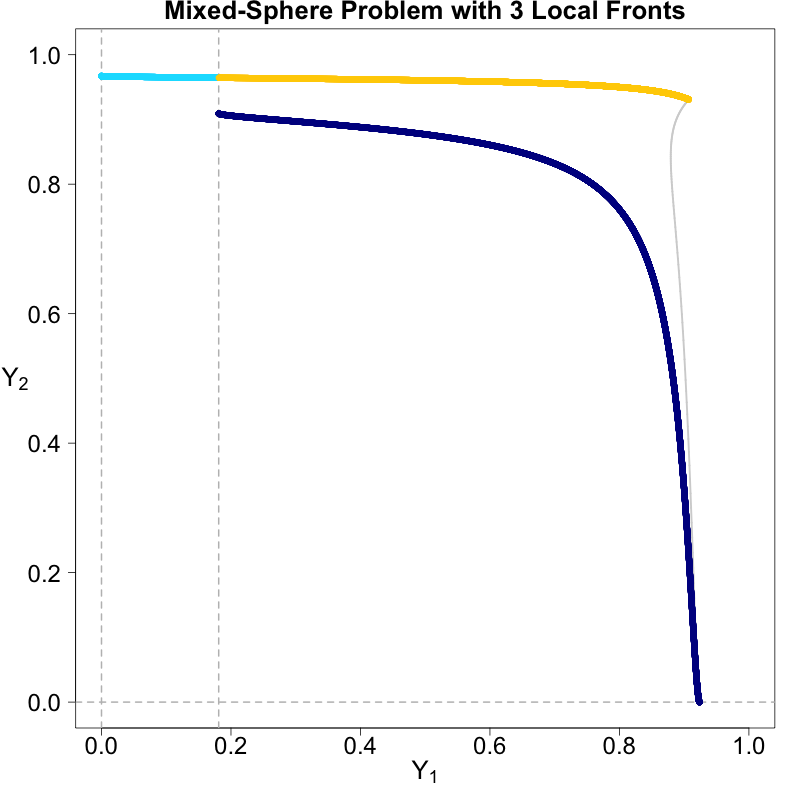
- Heatmap:
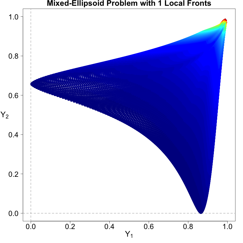
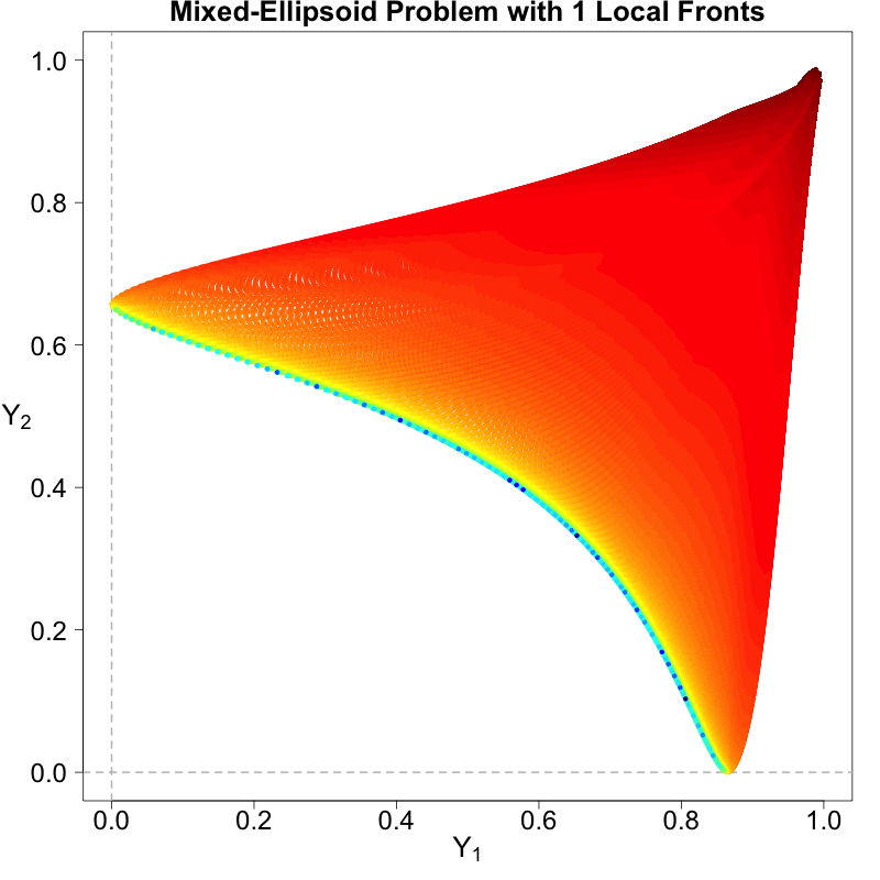
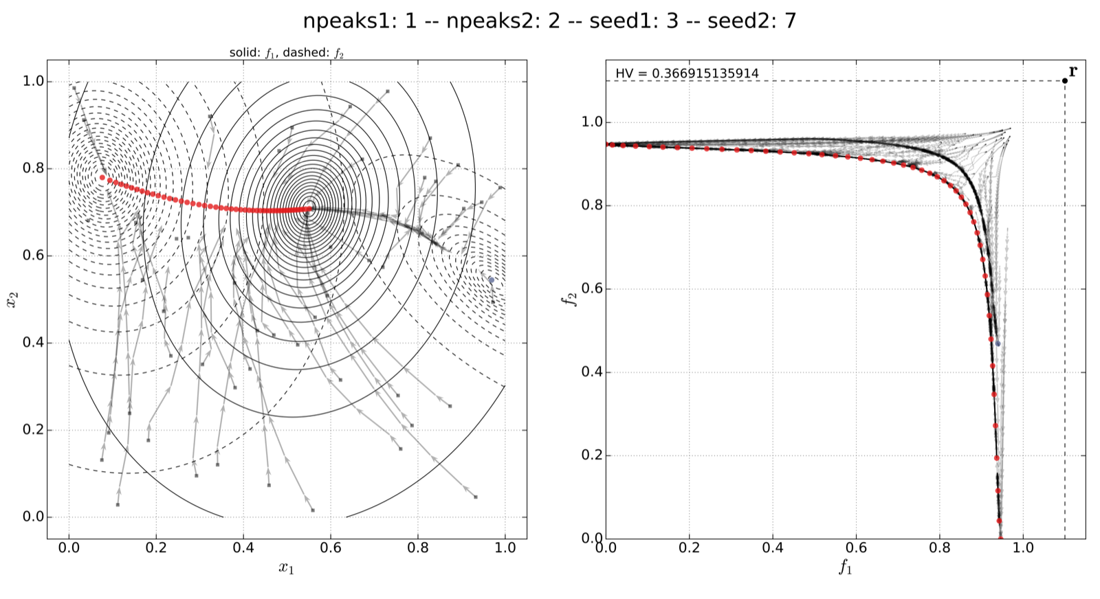
A heatmap visualizing the cumulated length of the gradient paths (either in a regular coloring scheme or based on a log-scale) - Objective Space:
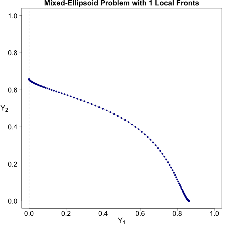
- theoretical:
The location of the theoretically true local efficient sets - regular / log-scale:
A mapping of the heatmap-coloring for each point from the decision space to the corresponding image in the objective space (using the coloring based on the actual cumulated path length or using a log-scaled version of the path lengths).
- theoretical:
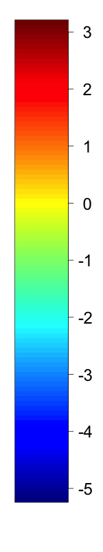
- Legend Color Bar:
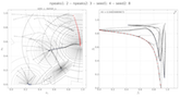
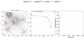
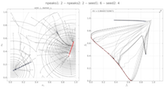
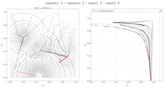
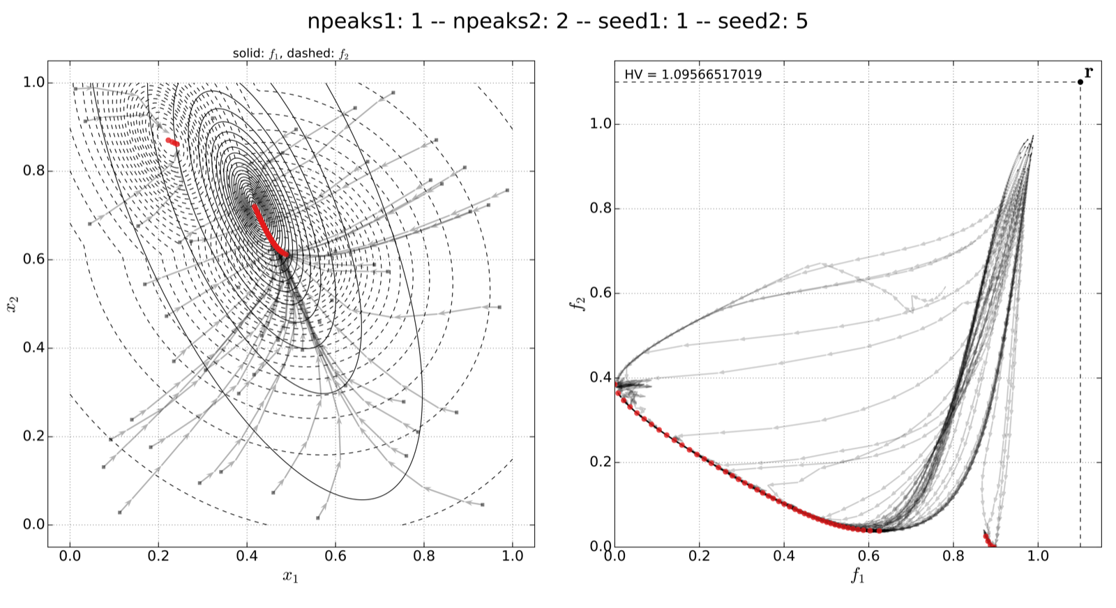
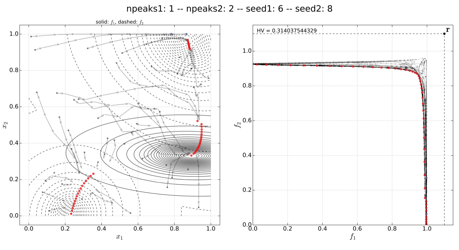
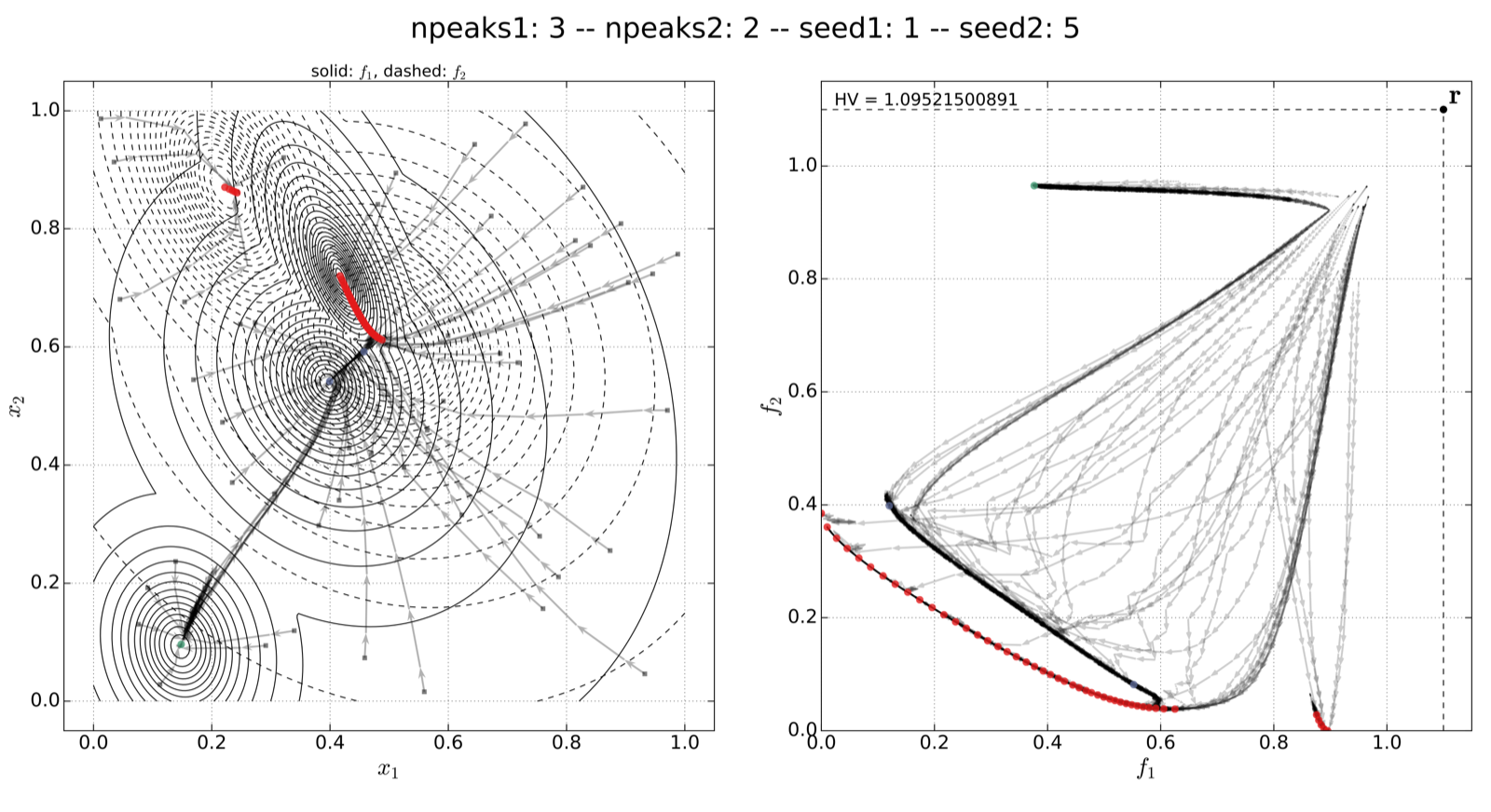
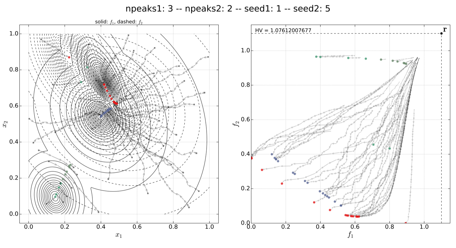
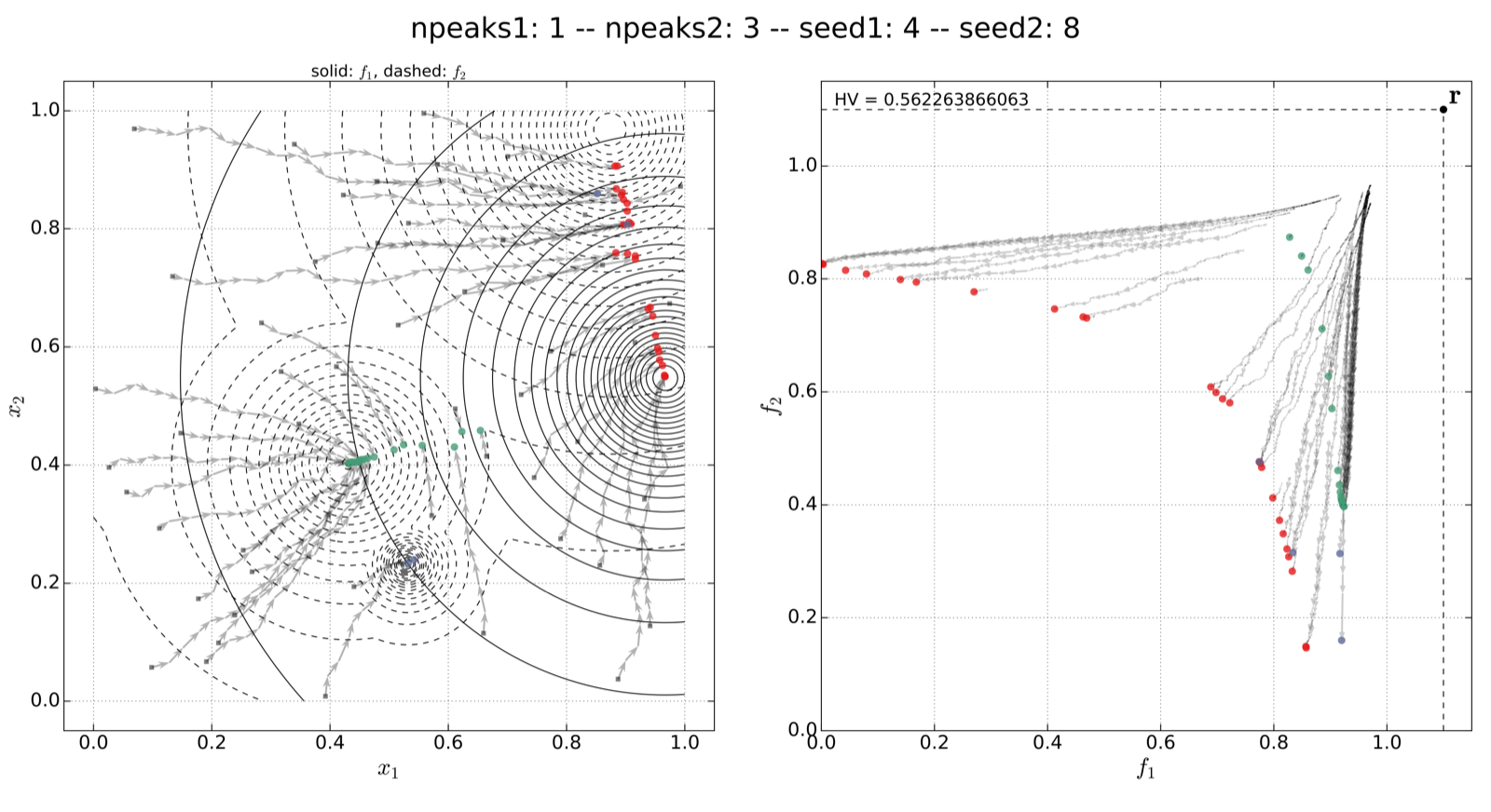
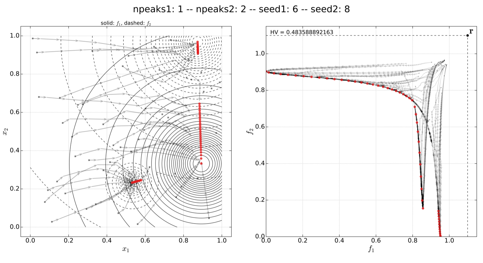
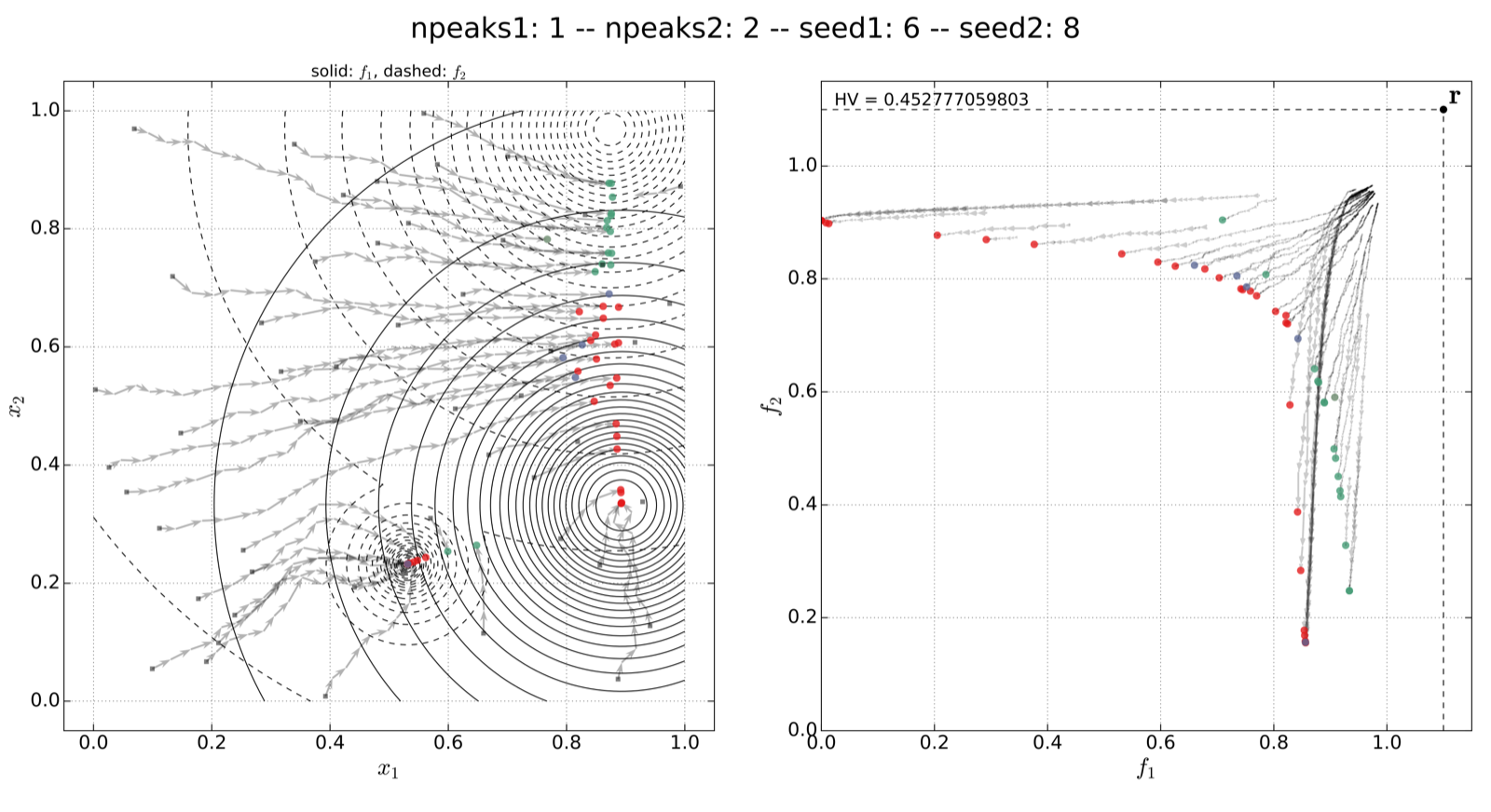
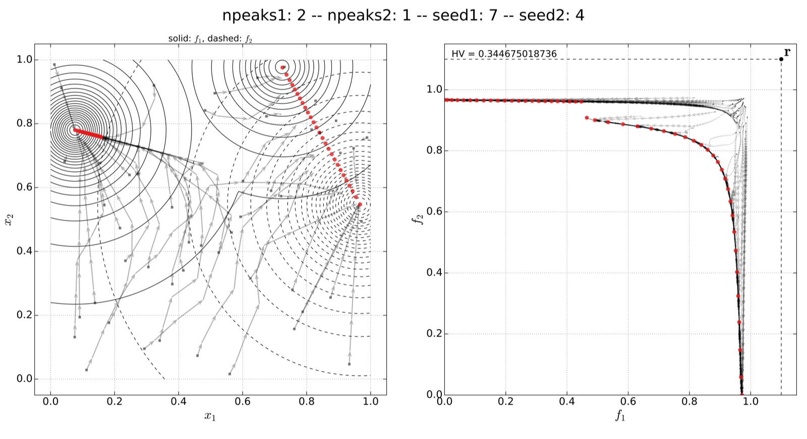
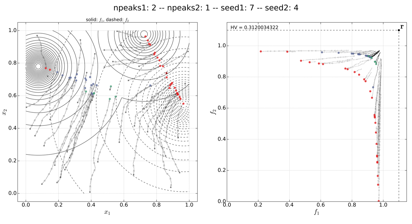
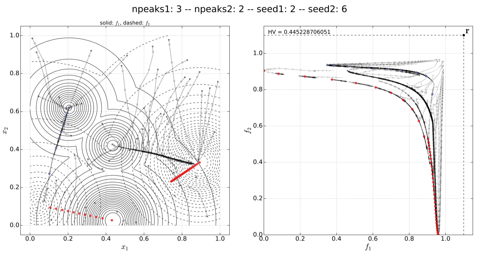
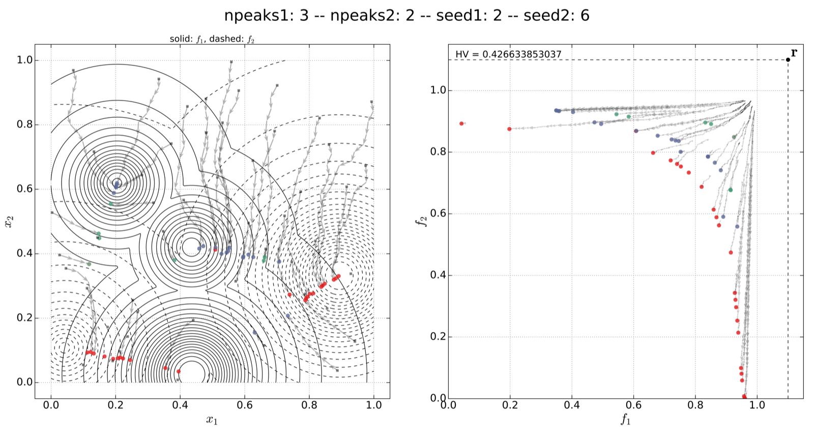
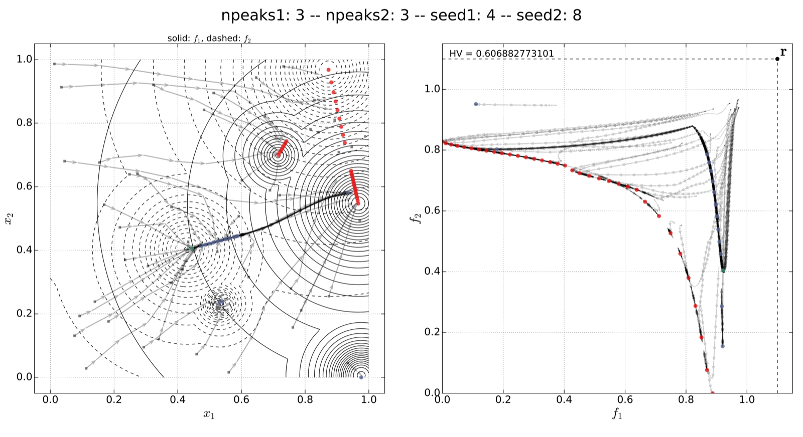
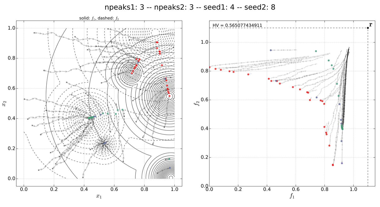
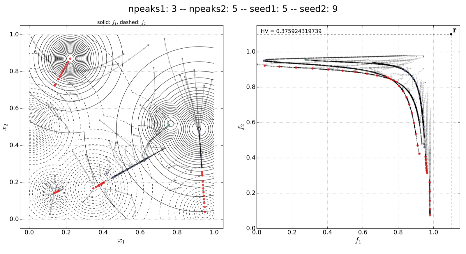
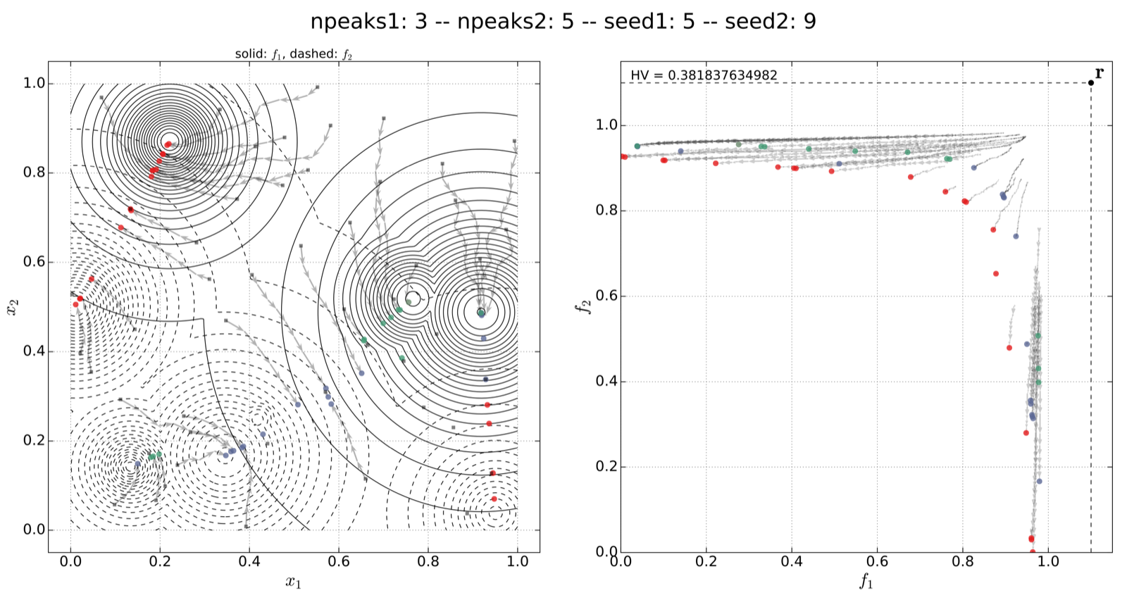
A legend of the coloring that was used within the heatmaps and/or the figures of the objective space. - Algorithm Behaviour:
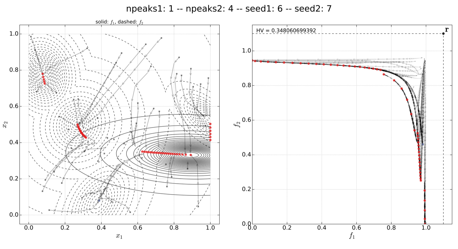
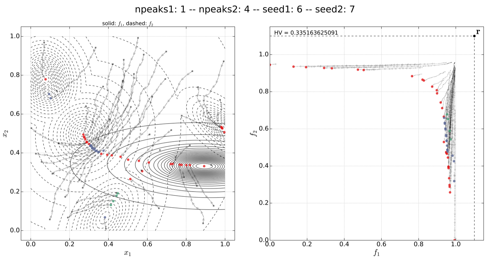
Trace of the population (shown within the decision and objective space) for two optimization algorithms (HIGA-MO and SLS). The traces are available as a png-image or a zipped movie.
- Heatmap:
ID Problem Setup Figures Movies
Shape of
PeaksRotate
PeaksProblem
DimensionTopology # Peaks Seed Heatmap Objective Space Legend Color Bar Algorithm Behavior Algorithm Behavior
f1 f2 f1 f2 regular log-scale theoretical regular log-scale regular log-scale HIGA-MO SLS HIGA-MO SLS
1 ellipse TRUE 2 random 1 1 1 3 


2 ellipse TRUE 2 random 1 2 1 5 


3 ellipse TRUE 2 random 1 2 2 6 


4 ellipse TRUE 2 random 1 2 3 7 


5 ellipse TRUE 2 random 1 3 4 8 


6 ellipse TRUE 2 random 1 5 5 9 


7 ellipse TRUE 2 random 1 2 6 8 


8 ellipse TRUE 2 random 1 4 6 7 


9 ellipse TRUE 2 random 2 2 1 5 


10 ellipse TRUE 2 random 2 2 2 6 


11 ellipse TRUE 2 random 2 2 3 7 


12 ellipse TRUE 2 random 2 3 4 8 


13 ellipse TRUE 2 random 2 5 5 9 


14 ellipse TRUE 2 random 2 2 6 4 


15 ellipse TRUE 2 random 2 1 7 4 


16 ellipse TRUE 2 random 3 2 1 5 


17 ellipse TRUE 2 random 3 2 2 6 


18 ellipse TRUE 2 random 3 2 3 7 


19 ellipse TRUE 2 random 3 3 4 8 


20 ellipse TRUE 2 random 3 5 5 9 


21 sphere FALSE 2 random 1 1 1 3 


22 sphere FALSE 2 random 1 2 1 5 


23 sphere FALSE 2 random 1 2 2 6 


24 sphere FALSE 2 random 1 2 3 7 


25 sphere FALSE 2 random 1 3 4 8 


26 sphere FALSE 2 random 1 5 5 9 


27 sphere FALSE 2 random 1 2 6 8 


28 sphere FALSE 2 random 1 4 6 7 


29 sphere FALSE 2 random 2 2 1 5 


30 sphere FALSE 2 random 2 2 2 6 


31 sphere FALSE 2 random 2 2 3 7 


32 sphere FALSE 2 random 2 3 4 8 


33 sphere FALSE 2 random 2 5 5 9 


34 sphere FALSE 2 random 2 2 6 4 


35 sphere FALSE 2 random 2 1 7 4 


36 sphere FALSE 2 random 3 2 1 5 


37 sphere FALSE 2 random 3 2 2 6 


38 sphere FALSE 2 random 3 2 3 7 


39 sphere FALSE 2 random 3 3 4 8 


40 sphere FALSE 2 random 3 5 5 9 


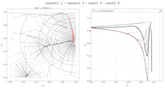
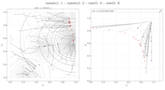
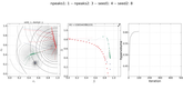
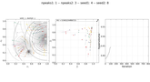
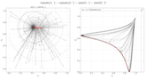
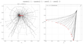
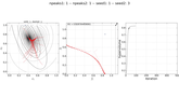
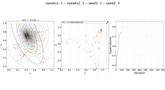
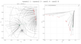
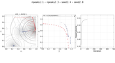
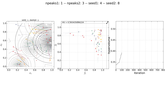
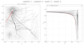
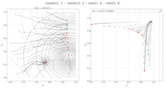
In addition to the visual results shown above, we also computed problem characteristics (so to say, "white-box landscape features"), as well as algorithm characteristics (for HIGA-MO and SLS) for each of the 40 benchmark instances. Based on these problem and lanscape characteristics, we performed a principal component analysis (PCA) and had a look at the respective biplots: one biplot across all characteristics, one for the problem characteristcs, one for the algorithm characteristics of HIGA-MO and one for the ones of SLS.


-
 Algorithm Selection on Traveling Salesperson Problems (TSP)
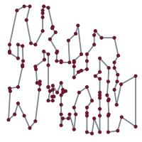
This is joint work of members from our group (Information Systems and Statistics) and colleagues from the Computer Science Department of the University of British Columbia.
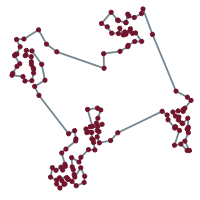
As a first result of this fruitful collaboration, we have published a paper on "Improving the State of the Art in Inexact TSP Solving using Per-Instance Algorithm Selection" at the Learning and Intelligent OptimizatioN Conference (LION9) in Lille, France. Furthermore, we have implemented two R-packages that on the one hand provide the methods for generating clustered TSP instances (netgen) and on the other hand offer a comprehensive toolbox for solving and analyzing symmetric Travelling Salesperson Problems (salesperson).
In August 2017, our paper on "Leveraging TSP Solver Complementarity through Machine Learning" has been accepted for publication in the Evolutionary Computation Journal (ECJ).
Further information on this very interesting topic can be found on our project's website.